Notes / 2025-12-01

Similar-Day Naive Method

Like the Chronos-2 technical report, Uniejewski and Weron compare the approaches implemented in their aforementioned paper against a naive baseline. Unlike the technical report which uses seasonal naive for all data sets, Uniejewski and Weron, to their credit, employ a baseline that, while naive, is tuned to their use case of electricity price forecasting and employs as much knowledge as possible:

The first benchmark, the so-called naive method, belongs to the class of similar-day techniques. It is defined by $\hat{P}_{d,h} = \hat{P}_{d-7,h}$ for Monday, Saturday and Sunday, and $\hat{P}_{d,h} = \hat{P}_{d-1,h}$ otherwise. As Contreras et al. argued, forecasting procedures that are not calibrated carefully fail to outperform this extremely simple method surprisingly often.

So given the different human patterns in electricity usage on workdays and on weekends, they use the naive method for workdays and seasonal naive for the weekend and Monday (because Sunday can’t be used to predict Monday).

Reminds me of this footnote.

Notes / 2025-11-30

Scaling Time Series Using the Inverse Hyperbolic Sine

This one’s new to me: The Chronos-2 tokenization pipeline follows up an initial standardization of input time series with a variance stabilizing transformation in the inverse hyperbolic sine function, $\sinh^{-1}$, as described in the model’s technical report.

The inverse hyperbolic sine function is defined as:

As such it is an alternative to the $\ln(x+1)$ transform with the added benefit of being applicable to negative values.

While news to me, the technical report points out that the inverse hyperbolic sine is no news to the electricity price forecasting literature, citing “Efficient Forecasting of Electricity Spot Prices with Expert and LASSO Models” by Bartosz Uniejewski and Rafał Weron, which describes the inverse hyperbolic sine and other variance stabilizing transformations in more detail.

Notes / 2025-11-23

Stacking Simple Forecasts by Classification

This paper got me thinking about stacking and ensembling of forecasts again.

Different from what the paper proposes but in the stacking models-sense, consider some multi-class classification model used to predict which base model forecasts a given observation from a set of many time series best. Something more akin to the FFORMA approach.

But use simple forecast methods to keep the overhead of first creating base forecasts at a minimum. Use the seasonal lag, the seasonal average, the most recent observation, zero, year-to-date average, etc. as base forecasts. Anything, really, that makes for a strong baseline for part of your dataset and can be calculated “without training”. If nothing else, this avoids the need for expensive cross-validation loads (as those described in the aforementioned paper).

Then, for each observation of your time series data, derive a label based on the base forecast that comes closest to the observation.¹

Finally, train the classifer model to predict the labels, using the base models as features, but also any other kind of feature. Now well and truly spitballing: Have some features summarize base predictions relative to one another, and relative to recent observations (“The seasonal lag is 190% of the year-to-date average”) to help the model distinguish patters.

Given that the classifier model would only pick between simple forecast methods to arrive at the final prediction, the overall forecast accuracy will always be limited. I can imagine scenarios, however, where the prediction ends up being more stable and at the right level compared to models trained to predict the time series directly. Constrained by the quality of the base forecasts, this stacking approach could pay off handsomely if the optimal base learner differs across the set of time series, or frequently changes within the same series. That is, when there is no dominant baseline.

For example, it could work well in scenarios where time series have multi-modal distributions due to zeroes, or frequently exhibit structural breaks.

In a way, the classifier would learn the sort of “item routing” described here. Instead of assigning time series to different forecast models based on rules, the classifier will split the data into subsets and assign the model.

One more nice side effect: There is no need for target scaling when base forecasts are non-trained methods and when the meta learner only needs to classify.

The overall approach is also fairly explainable if not interpretable. Especially if one picks the features for additional context wisely.

Finally, while the base forecasts will limit the overall forecast quality that can be achieved, we can measure the best possible forecast quality the stacking approach can reach in the hypothetical case of a perfect classification of every observation. So before putting any effort into training a good classifier, we will know whether the effort could hypothetically be worth it.

Though there is a limit to the number of base forecasts you should use to derive the labels for the classifier. Dare to use the range of real numbers and you’ll end up back with a (discretized) regression problem.

Notes / 2025-03-16

Inherently Coherent Forecasts

Suppose you offer a single API endpoint that takes historical observations of one time series at a time (not unlike Nixtla’s TimeGPT). Suppose further that everyone at your company uses this endpoint to generate any business forecast they need. What behaviors should the API’s forecast exhibit?

An obvious one would be forecast coherence across aggregation levels. Say your company sells three products. You have the historical revenue for the three products, $Y_1$, $Y_2$, $Y_3$, as well as the historical revenue for the company as a whole, $Y$, where $Y=Y_1+Y_2+Y_3$. When you feed $Y_1$ into the API, the API returns forecast $\text{API}(Y_1)=\hat{Y}_1$. It returns $\hat{Y}_2$ given $Y_2$, $\hat{Y}_3$ given $Y_3$, and given $Y$ it returns $\hat{Y}$. If we want to see a forecast at company-level that “makes sense” given product-level forecasts, we want the forecasts to be coherent: $\hat{Y}=\hat{Y}_1 + \hat{Y}_2 + \hat{Y}_3$. But given that the API only ever sees one time series at a time, what model could be used to provide coherent forecasts?

Again, keep in mind that the API doesn’t have access to more information than its current input. For example, when you feed it $Y_2$, it doesn’t know that $Y_1$ and $Y_3$ exist. It also doesn’t know whether $Y_2$ is at the hierarchy’s bottom- or top-level. The API does not have access to all possible time series that exist at the company. Consequently, the API does not have the information required to apply the methods from the vast literature on coherent forecasts. What modeling approach will return coherent forecasts nevertheless?

The seasonal naive method would. As would the naive method, of course. The mean forecast, too. And any other linear combination of the past observations with a pre-determined context length and coefficients.¹ Any pre-trained—the coefficients must not change depending on the input provided to the API—linear autoregressive model of order p will do.

That’s a fairly flexible model family. It also includes the Non-Parametric Time Series Forecaster and Threedx. Thus, the API could do an OK job for most series passed to it. It would have an obvious weakness in new or recently discontinued time series, though. The API could not, for example, override its usual forecast for a recently discontinued product and forecast zero instead. The same holds for any other kind of structural break as well as anomalies. That would make it tough to rely exclusively on such an API for operational decisions happening at the low hierarchy level ridden with discontinuities.

The above combined with recent evidence make me inclined to offer the seasonal naive method as Zero-Shot Foundation Model with Inherently Coherent Forecasts available as API.

Notes / 2025-01-12

R-squared as Forecast Evaluation Metric

When Jane Street’s \$120,000 “Real-Time Market Data Forecasting” Kaggle competition closes tomorrow, submitted forecasts will be evaluated using $R^2$:

Submissions are evaluated on a scoring function defined as the sample weighted zero-mean R-squared score ($R^2$) of responder_6. The formula is give by: $R^2 = 1 - \frac{\sum w_i(y_i - \hat{y}_i)^2}{\sum w_i y_i^2}$ where $y$ and $\hat{y}$ are the ground-truth and predicted value vectors of responder_6, respectively; $w$ is the sample weight vector.

Stats 101 courses have left $R^2$ with a bad rep as gameable regression metric. But I’ve come to appreciate it as a metric in forecasting—when calculated on the test set with the total-sum-of-squares denominator based on the test period’s empirical mean, $\bar{y}_{T,h} = \sum_{t = T+1}^{T+h}y_t$, where $T$ is the training set’s last observation and $h$ the number of observations in the test set. Then:

Above definition gives the total-sum-of-squares the advantage of future knowledge included in $\bar{y}_{T,h}$ that the predictions $\hat{y}_t$ used for the residual-sum-of-squares do not have. In comparison to its linear regression origin, this test set-focused definition is not going to improve as parameters are added to the forecast model. But it does keep its interpretability:

• A value of 1 indicates a perfect model
• A value of 0 indicates a model as good as the test mean (the latter being a forecast that is both perfectly unbiased and perfectly predicts the total sum over the forecast horizon)
• Any negative value indicates a model that isn’t even as good as the simple test mean (but then again, the test mean uses future knowledge)

For example, when predicting the final twelve months of AirPassengers data, the obviously poor prediction given by the training set mean results in an $R^2$ of -8.24 whereas a seasonal naive prediction achieves an $R^2$ of 0.54.

This shouldn’t come as a suprise. Interpreting $R^2$ as the fraction of (test) variance explained, the seasonal naive prediction can explain more than half of the variance that the test mean left unexplained. The model captures a large part of the signal hidden in the data’s variation.

Just like Jane Street replaced the test set empirical mean in their definition of $R^2$ by zero, which in their application of predicting expected financial returns is a hard to beat expected value, one could replace the total sum of squares denominator by the squared errors of a different benchmark such as seasonal naive predictions when it is known that due to the data’s seasonality the seasonal naive prediction will consistently outperform the test set mean despite its future knowledge. Thus, $R^2$ is not so different from the more common relative measures such as the Relative Mean Squared Error described in section 6.1.4 of Hewamalage et al. (2022), or Skill Scores employed in weather prediction described by Murphy (1988).

Then again, when a time series’ variance is not dominated by its seasonal component, $R^2$ and its interpretation as fraction of variance explained can leave a damning picture of a model’s forecasts not actually being all that skillful. It casts doubt by asking how much signal your model has picked up to meaningfully predict future variation. Suddenly any value larger than zero will feel like an enormous success.

Notes / 2024-04-21

Debug Forecasts with Animated Plots

Speaking of GIFs, animated visualizations of rolling forecasts are eye-opening to the impact of individual observations, the number of observations, and default settings on a model’s forecasts. In the example below, the default forecast::auto.arima() transitions between poor model specifications until it can finally pick up the seasonality after 24 observations, only to generate a negative point forecast despite purely non-negative observations.

Fantastic way to understand forecast methods’ edge-case behavior.

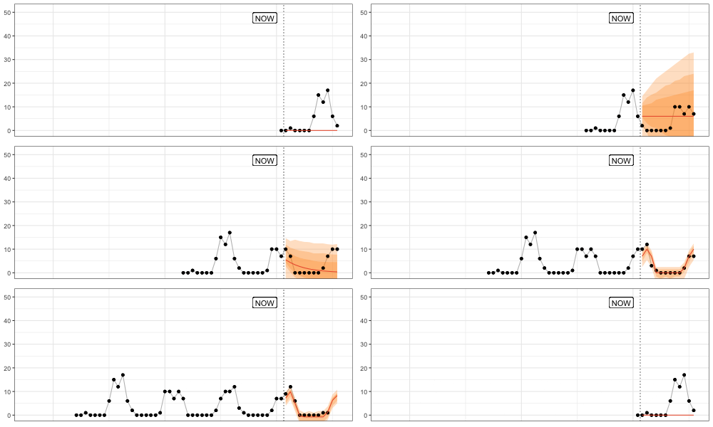
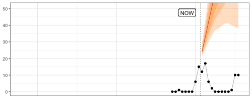
My favorite frame? After nine observations, when a model specification with trend is picked and returns an exploding forecast based on very little evidence.

The code for this GIF in this small Github repo.

Notes / 2023-12-12

Stop Using Dynamic Time Warping for Business Time Series

Dynamic Time Warping (DTW) is designed to reveal inherent similarity between two time series of similar scale that was obscured because the time series were shifted in time or sampled at different speeds. This makes DTW useful for time series of natural phenomena like electrocardiogram measurements or recordings of human movements, but less so for business time series such as product sales.

To see why that is, let’s first refresh our intuition of DTW, to then check why DTW is not the right tool for business time series.

What Dynamic Time Warping Does

Given two time series, DTW computes aligned versions of the time series to minimize the cumulative distance between the aligned observations. The alignment procedure repeats some of the observations to reduce the resulting distance. The aligned time series end up with more observations than in the original versions, but the aligned versions still have to have the same start and end, no observation may be dropped, and the order of observations must be unchanged.

But the best way to understand the alignment is to visualize it.

Aligning a Shift

To start, I’ll use an example where DTW can compute a near perfect alignment: That of a cosine curve and a shifted cosine curve—which is just a sine curve.¹ For each of the curves, we observe 12 observations per period, and 13 observations in total.

series_sine <- sinpi((0:12) / 6)
series_cosine <- cospi((0:12) / 6)

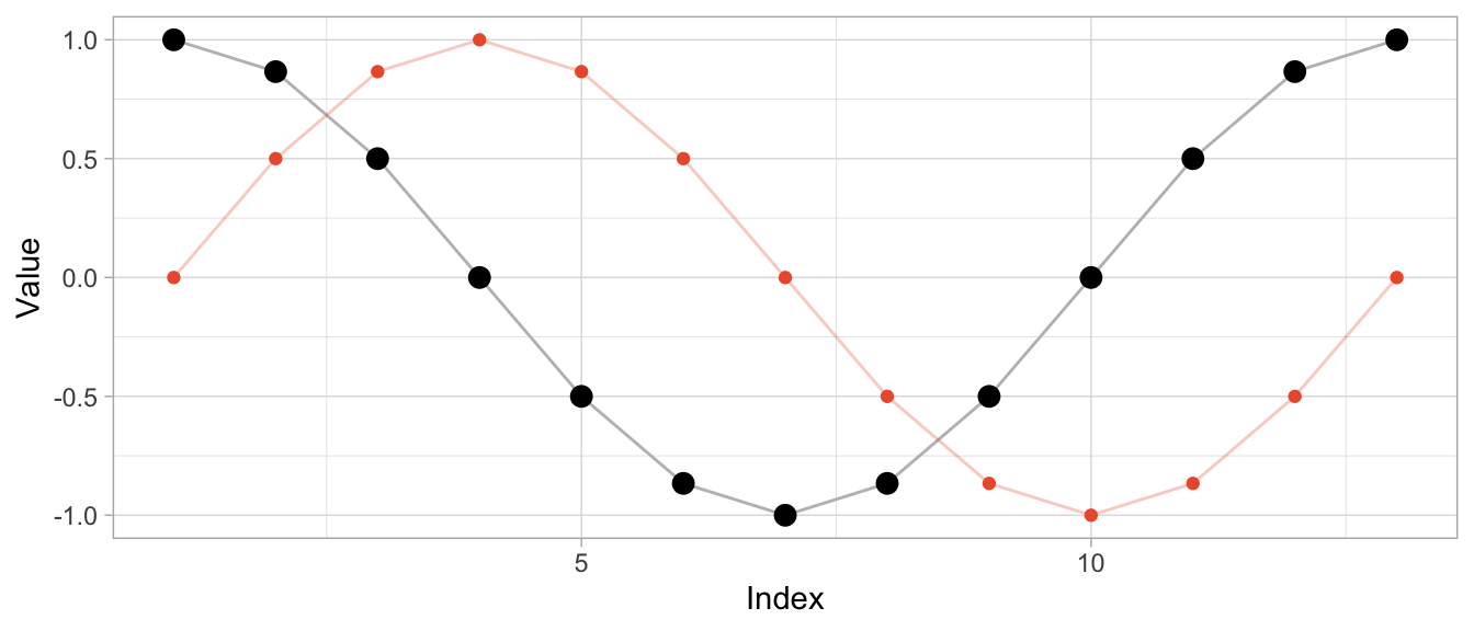
To compute the aligned versions, I use the DTW implementation of the dtw package (also available for Python as dtw-python) with default parameters.

library(dtw)
dtw_shift <- dtw::dtw(x = series_sine, y = series_cosine)

Besides returning the distance of the aligned series, DTW produces a mapping of original series to aligned series in the form of alignment vectors dtw_shift$index1 and dtw_shift$index2. Using those, I can visualize both the original time series and the aligned time series along with the repetitions used for alignment.

# DTW returns a vector of indices of the original observations
# where some indices are repeated to create aligned time series
dtw_shift$index2

##  [1]  1  1  1  1  2  3  4  5  6  7  8  9 10 11 12 13

# In this case, the first index is repeated thrice so that the first
# observation appears four times in the aligned time series
series_cosine[dtw_shift$index2] |> head(8) |> round(2)

## [1]  1.00  1.00  1.00  1.00  0.87  0.50  0.00 -0.50

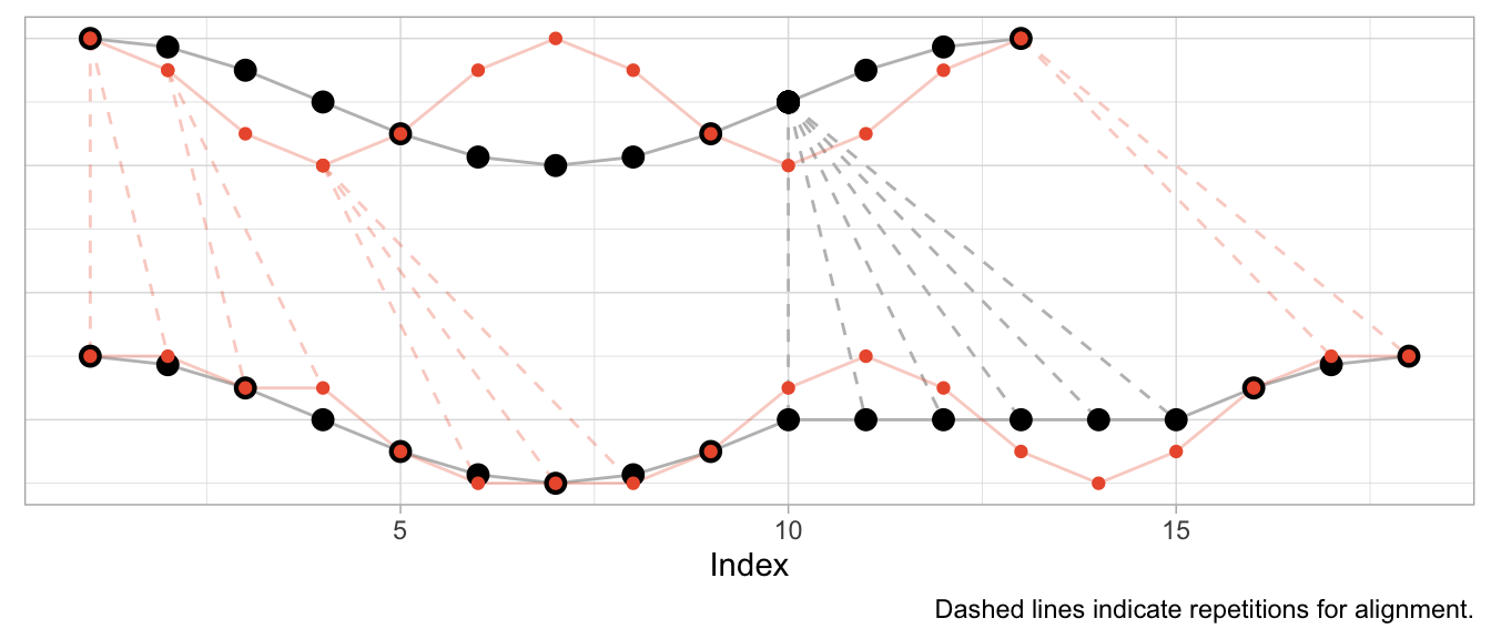
The plot below shows the original time series in the upper half and the aligned time series in the lower half, with the sine in orange and the cosine in black. Dashed lines indicate where observations were repeated to achieve the alignment.

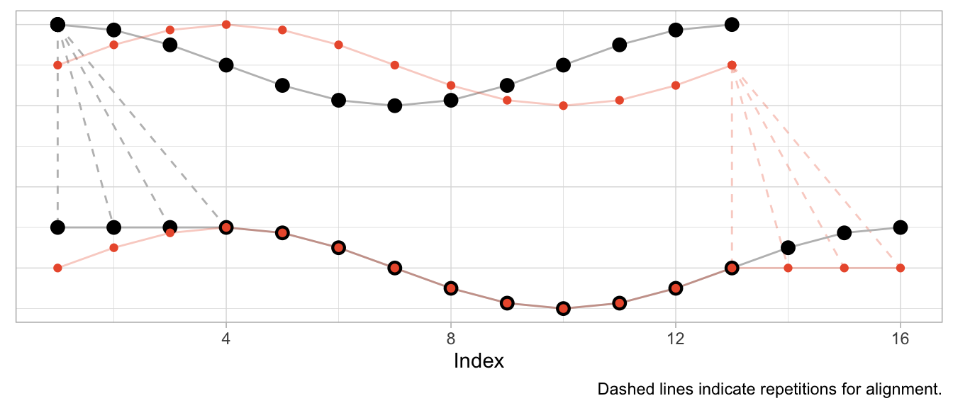
Given that the sine is a perfect shifted copy of the cosine, three-quarters of the observed period can be aligned perfectly. The first quarter of the sine and the last quarter of the cosine’s period, however, can’t be aligned and stand on their own. Their indices are mapped to the repeated observations from the other time series, respectively.

Aligning Speed

Instead of shifting the cosine, I can sample it at a different speed (or, equivalently, observe a cosine of different frequency) to construct a different time series that can be aligned well by DTW. In that case, the required alignment is not so much a shift as it is a squeezing and stretching of the observed series.

Let’s create a version of the original cosine that is twice as “fast”: In the time that we observe one period of the original cosine, we observe two periods of the fast cosine.

series_cosine_fast <- cospi((0:12) / 3)
dtw_fast <- dtw::dtw(x = series_cosine_fast, y = series_cosine)

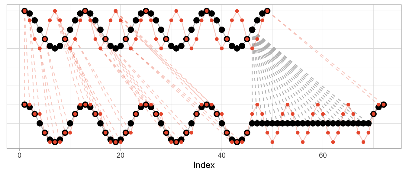
The resulting alignment mapping looks quite different than in the first example. Under a shift, most observations still have a one-to-one mapping after alignment. Under varying frequencies, most observations of the faster time series have to be repeated to align. Note how the first half of the fast cosine’s first period can be neatly aligned with the first half of the slow cosine’s period by repeating observations (in an ideal world exactly twice).

The kind of alignment reveals itself better when the time series are observed for more than just one or two periods. Below, for longer versions of the same series, half of the fast time series can be matched neatly with the slow cosine as we observe twice the number of periods for the fast cosine.

Aligning Different Scales

What’s perhaps unexpected, though, is that the alignment works only on the time dimension. Dynamic time warping will not scale the time series’ amplitude. But at the same time DTW is not scale independent. This can make the alignment fairly awkward when time series have varying scales as DTW exploits the time dimension to reduce the cumulative distance of observations in the value dimension.

To illustrate this, let’s take the sine and cosine from the first example but scale the sine’s amplitude by 5 and check the resulting alignment.

series_sine_scaled <- series_sine * 10
dtw_scaled <- dtw::dtw(x = series_sine_scaled, y = series_cosine)

We might expect DTW to align the two series as it did in the first example above with unscaled series. After all, the series have the same frequencies as before and the same period shift as before.

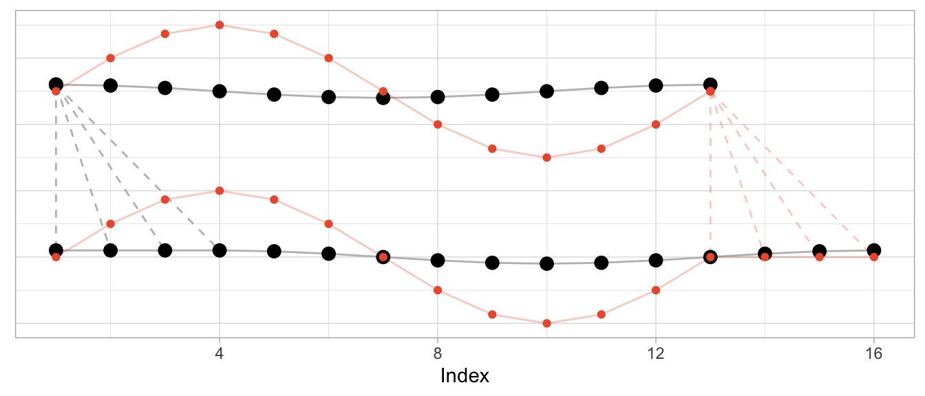
This is what the alignment would look like using the alignment vectors from the first example above based on un-scaled observations. While it’s a bit hard to see due to the different scales, the observations at peak amplitude are aligned (e.g., indices 4, 10, 16) as are those at the minimum amplitude (indices 7 and 13).

But Dynamic Time Warping’s optimization procedure doesn’t actually try to identify characteristics of time series such as their period length to align them. It warps time series purely to minimize the cumulative distance between aligned observations. This may lead to a result in which also the periodicity is aligned as in the first and second examples above. But that’s more by accident than by design.

This is how DTW actually aligns the scaled sine and the unscaled cosine:

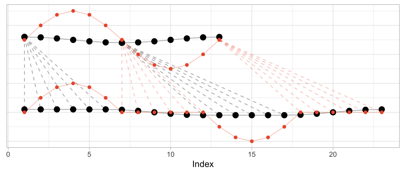
The change in the series’ amplitude leads to a more complicated alignment: Observations at the peak amplitude of the cosine (which has the small amplitude) are repeated many times to reduce the Euclidean distance to the already high amplitude observations of the sine. Reversely, the minimum-amplitude of the sine is repeated many times to reduce the Euclidean distance to the already low amplitude observations of the cosine.

DTW Is Good at Many Things…

Dynamic time warping is great when you’re observing physical phenomena that are naturally shifted in time or at different speeds.

Consider, for example, measurements taken in a medical context such as those of an electrocardiogram (ECG) that measures the electrical signals in a patient’s heart. In this context, it is helpful to align time series to identify similar heart rhythms across patients. The rhythms’ periods could be aligned to check whether one patient has the same issues as another. Even for the same person a DTW can be useful to align measurements taken on different days at different heart rates.

data("aami3a") # ECG data included in `dtw` package
dtw_ecg <- dtw::dtw(
  x = as.numeric(aami3a)[1:2880],
  y = as.numeric(aami3a)[40001:42880]
)

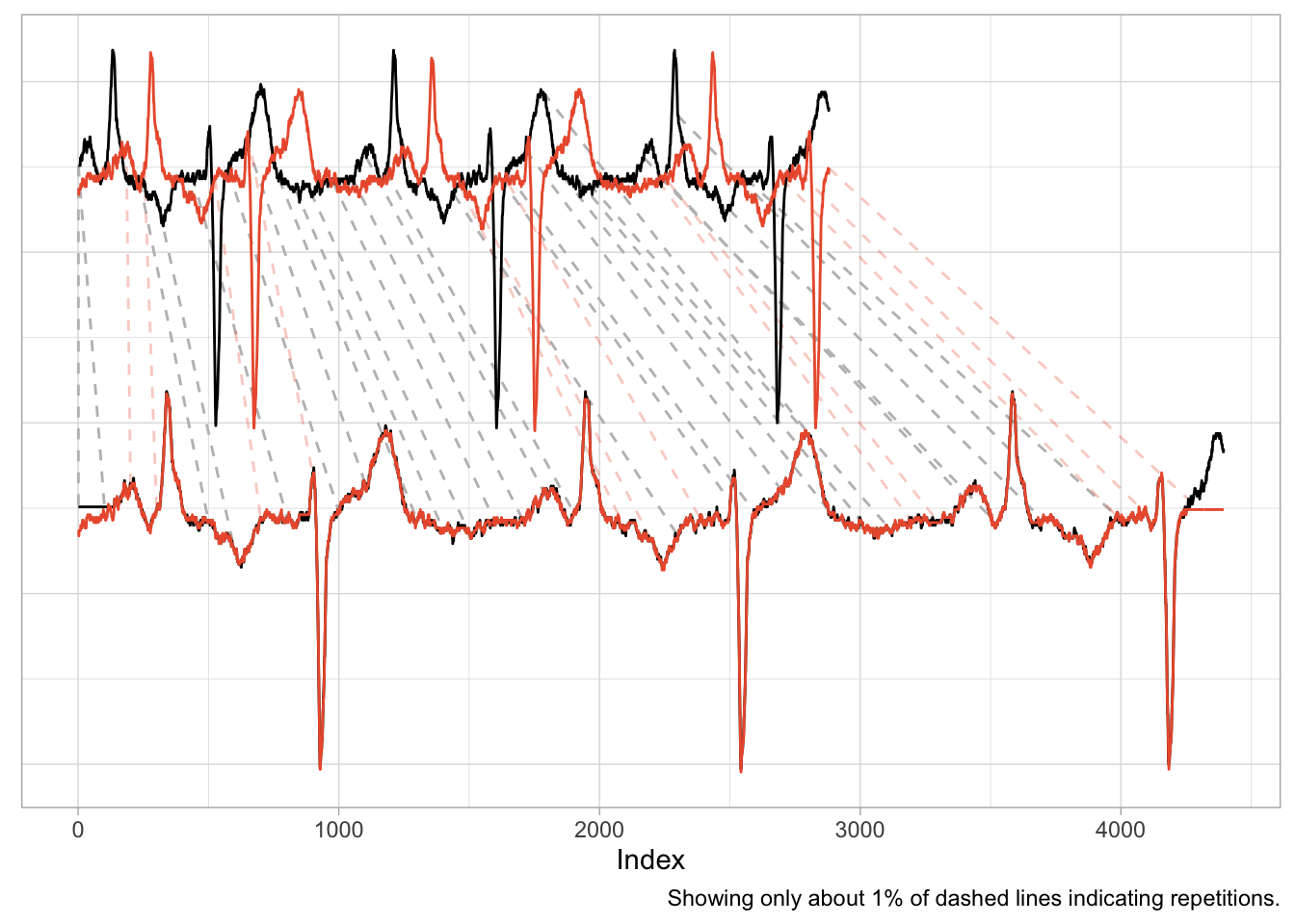
An application such as this one is nearly identical to the first example of the shifted cosine. And as the scale of the time series is naturally the same across the two series, the alignment works well, mapping peaks and valleys with minimal repetitions.

There is also a natural interpretation to the alignment, namely that we are aligning the heart rhythm across measurements. A large distance after alignment would indicate differences in rhythms.

…But Comparing Sales Ain’t One of Them

It is enticing to use Dynamic Time Warping in a business context, too. Not only does it promise a better distance metric to identify time series that are “similar” and to separate them from those that are “different”, but it also has a cool name. Who doesn’t want to warp stuff?

We can, for example, warp time series that count the number of times products are used for patients at a hospital per month. Not exactly product sales but sharing the same characteristics. The data comes with the expsmooth package.

set.seed(47772)
sampled_series <- sample(x = ncol(expsmooth::hospital), size = 2)
product_a <- as.numeric(expsmooth::hospital[,sampled_series[1]])
product_b <- as.numeric(expsmooth::hospital[,sampled_series[2]])

While product_b is used about twice as often as product_a, both products exhibit an increase in their level at around index 40 which is perhaps one characteristic that makes them similar or at least more similar compared to a series that doesn’t share this increase.

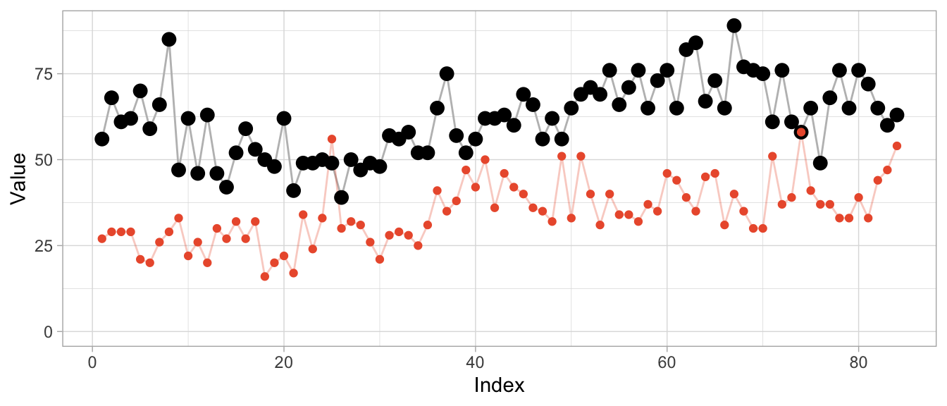
However, the warped versions exhibit a lot of unwanted repetitions of observations. Given the different level of the products, this should not come as a surprise.

dtw_products_ab <- dtw::dtw(x = product_b, y = product_a)

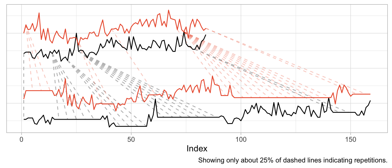
We can mostly fix this by min-max scaling the series, forcing their observations onto the same range of values.

dtw_products_ab_standardized <- dtw::dtw(
  x = (product_b - min(product_b)) / (max(product_b) - min(product_b)),
  y = (product_a - min(product_a)) / (max(product_a) - min(product_a))
)

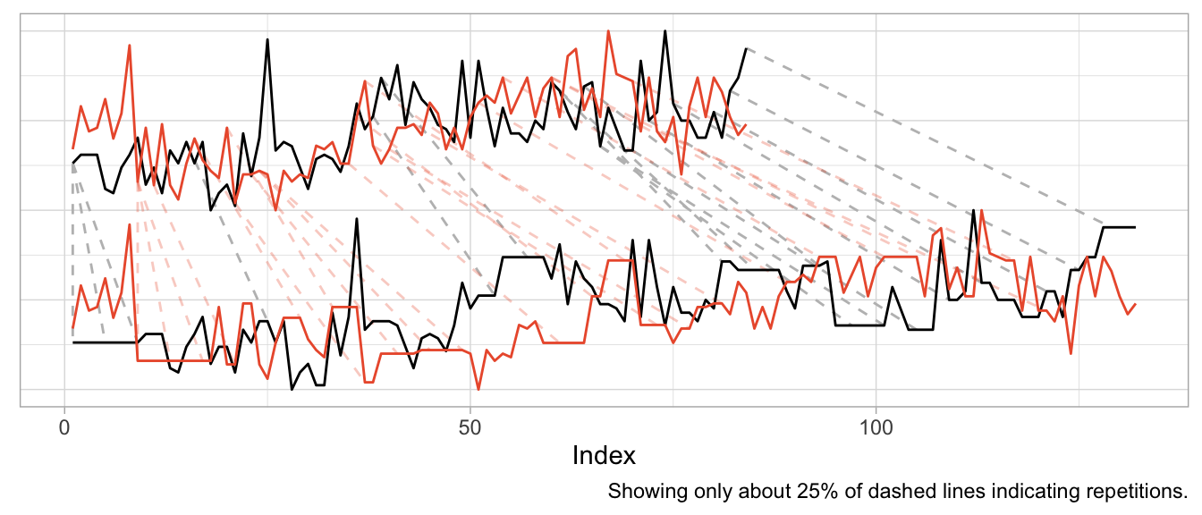
While we got rid of the unwanted warping artifacts in the form of extremely long repetitions of the same observation, the previous plot should raise some questions:

• How can we interpret the modifications for “improved” alignment?
• Are we aligning just noise?
• What does the warping offer us that we didn’t already have before?

If you ask me, there is no useful interpretation to the alignment modifications, because the time series already were aligned. Business time series are naturally aligned by the point in time at which they are observed.²

We also are not taking measurement of a continuous physical phenomenon that goes up and down like the electric signals in a heart. While you can double the amount of ECG measurements per second, it does not make sense to “double the amount of sales measurements per month”. And while a product can “sell faster” than another, this results in an increased amplitude not an increased frequency (or shortened period lengths).

So if you apply Dynamic Time Warping to business time series, you will mostly be warping random fluctuations with the goal of reducing the cumulative distance just that tiny bit more.

This holds when you use Dynamic Time Warping to derive distances for clustering of business time series, too. You might as well calculate the Euclidean distance³ on the raw time series without warping first. At least then the distance between time series will tell you that they were similar (or different) at the same point in time.

In fact, if you want to cluster business time series (or train any kind of model on them), put your focus on aligning them well in the value dimension by thinking carefully about how you standardize them. That makes all the difference.

Before using Dynamic Time Warping, ask yourself: What kind of similarity are you looking for when comparing time series? Will there be meaning to the alignment that Dynamic Time Warping induces in your time series? And what is it that you can do after warping that you weren’t able to do before?

Notes / 2023-12-03

Comes with Anomaly Detection Included

A powerful pattern in forecasting is that of model-based anomaly detection during model training. It exploits the inherently iterative nature of forecasting models and goes something like this:

1. Train your model up to time step t based on data [1,t-1]
2. Predict the forecast distibution at time step t
3. Compare the observed value against the predicted distribution at step t; flag the observation as anomaly if it is in the very tail of the distribution
4. Don’t update the model’s state based on the anomalous observation

For another description of this idea, see, for example, Alexandrov et al. (2019).

Importantly, you use your model to detect anomalies during training and not after training, thereby ensuring its state and forecast distribution are not corrupted by the anomalies.

The beauty of this approach is that

• the forecast distribution can properly reflect the impact of anomalies, and
• you don’t require a separate anomaly detection method with failure modes different from your model’s.

In contrast, standalone anomaly detection approaches would first have to solve the handling of trends and seasonalities themselves, too, before they could begin to detect any anomalous observation. So why not use the model you already trust with predicting your data to identify observations that don’t make sense to it?

This approach can be expensive if your model doesn’t train iteratively over observations in the first place. Many forecasting models¹ do, however, making this a fairly negligiable addition.

But enough introduction, let’s see it in action. First, I construct a simple time series y of monthly observations with yearly seasonality.

set.seed(472)
x <- 1:80
y <- pmax(0, sinpi(x / 6) * 25 + sqrt(x) * 10 + rnorm(n = 80, sd = 10))

# Insert anomalous observations that need to be detected
y[c(55, 56, 70)] <- 3 * y[c(55, 56, 70)]

To illustrate the method, I’m going to use a simple probabilistic variant of the Seasonal Naive method where the forecast distribution is assumed to be Normal with zero mean. Only the $\sigma$ parameter needs to be fitted, which I do using the standard deviation of the forecast residuals.

The estimation of the $\sigma$ parameter occurs in lockstep with the detection of anomalies. Let’s first define a data frame that holds the observations and will store a cleaned version of the observations, the fitted $\sigma$ and detected anomalies…

df <- data.frame(
  y = y,
  y_cleaned = y,
  forecast = NA_real_,
  residual = NA_real_,
  sigma = NA_real_,
  is_anomaly = FALSE
)

… and then let’s loop over the observations.

At each iteration, I first predict the current observation given the past and update the forecast distribution by calculating the standard deviation over all residuals that are available so far, before calculating the latest residual.

If the latest residual is in the tails of the current forecast distribution (i.e., larger than multiples of the standard deviation), the observation is flagged as anomalous.

For time steps with anomalous observations, I update the cleaned time series with the forecasted value (which informs a later forecast at step t+12) and set the residual to missing to keep the anomalous observation from distorting the forecast distribution.

# Loop starts when first prediction from Seasonal Naive is possible
for (t in 13:nrow(df)) {
  df$forecast[t] <- df$y_cleaned[t - 12]
  df$sigma[t] <- sd(df$residual, na.rm = TRUE)
  df$residual[t] <- df$y[t] - df$forecast[t]
  
  if (t > 25) {
	# Collect 12 residuals before starting anomaly detection
	df$is_anomaly[t] <- abs(df$residual[t]) > 3 * df$sigma[t]
  }
  
  if (df$is_anomaly[t]) {
	df$y_cleaned[t] <- df$forecast[t]
	df$residual[t] <- NA_real_
  }
}

Note that I decide to start the anomaly detection not before there are 12 residuals for one full seasonal period, as the $\sigma$ estimate based on less than a handful of observations can be flaky.

In a plot of the results, the combination of 1-step-ahead prediction and forecast distribution is used to distinguish between expected and anomalous observations, with the decision boundary indicated by the orange ribbon. At time steps where the observed value falls outside the ribbon, the orange line indicates the model prediction that is used to inform the model’s state going forward in place of the anomaly.

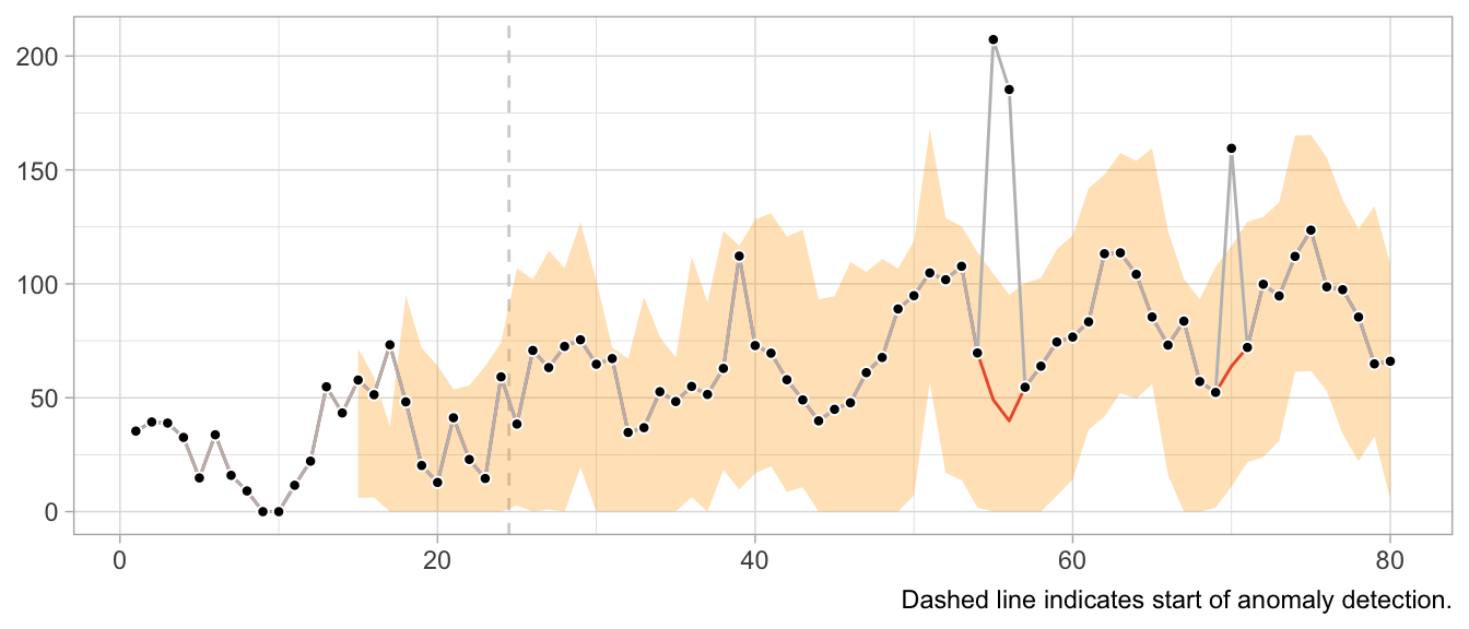
Note how the prediction at time t is not affected by the anomaly at time step t-12. Neither is the forecast distribution estimate.

This would look very different when one gets the update behavior slightly wrong. For example, the following implementation of the loop detects the first anomaly in the same way, but uses it to update the model’s state, leading to subsequently poor predictions and false positives, and fails to detect later anomalies.

# Loop starts when first prediction from Seasonal Naive is possible
for (t in 13:nrow(df)) {
  df$forecast[t] <- df$y[t - 12]
  df$sigma[t] <- sd(df$residual, na.rm = TRUE)
  df$residual[t] <- df$y[t] - df$forecast[t]
  
  if (t > 25) {
	# Collect 12 residuals before starting anomaly detection
	df$is_anomaly[t] <- abs(df$residual[t]) > 3 * df$sigma[t]
  }
  
  if (df$is_anomaly[t]) {
	df$y_cleaned[t] <- df$forecast[t]
  }
}

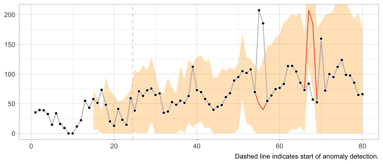
What about structural breaks?

While anomaly detection during training can work well, it may fail spectacularly if an anomaly is not an anomaly but the start of a structural break. Since structural breaks make the time series look different than it did before, chances are the first observation after the structural break will be flagged as anomaly. Then so will be the second. And then the third. And so on, until all observations after the structural break are treated as anomalies because the model never starts to adapt to the new state.

This is particularly frustrating because the Seasonal Naive method is robust against certain structural breaks that occur in the training period. Adding anomaly detection makes it vulnerable.

What values to use for the final forecast distribution?

Let’s get philosophical for a second. What are anomalies?

Ideally, they reflect a weird measurement that will never occur again. Or if it does, it’s another wrong measurement—but not the true state of the measured phenomenon. In that case, let’s drop the anomalies and ignore them in the forecast distribution.

But what if the anomalies are weird states that the measured phenomenon can end up in? For example, demand for subway rides after a popular concert. While perhaps an irregular and rare event, a similar event may occur again in the future. Do we want to exclude that possibility from our predictions about the future? What if the mention of a book on TikTok let’s sales spike? Drop the observation and assume it will not repeat? Perhaps unrealistic.

It depends on your context. In a business context, where measurement errors might be less of an issue, anomalies might need to be modeled, not excluded.

Notes / 2023-11-12

Code Responsibly

There exists this comparison of software before and software after machine learning.

Before machine learning, code was deterministic: Software engineers wrote code, the code included conditions with fixed thresholds, and at least in theory the program was entirely understandable.

After machine learning, code is no longer deterministic. Instead of software engineers instantiating it, the program’s logic is determined by a model and its parameters. Those parameters are not artisinally chosen by a software engineer but learned from data. The program becomes a function of data, and in some cases incomprehensible to the engineer due to the sheer number of parameters.

Given the current urge to regulate AI and making its use responsible and trustworthy, humans appear to expect machine learning models to introduce an obscene number of bugs into software. Perhaps humans underestimate the ways in which human programmers can mess up.

For example, when I hear Regulate AI, all I can think is Have you seen this stuff? By Pierluigi Bizzini for Algorithm Watch¹ (emphasis mine):

The algorithm evaluates teachers’ CVs and cross-references their preferences for location and class with schools’ vacancies. If there is a match, a provisional assignment is triggered, but the algorithm continues to assess other candidates. If it finds another matching candidate with a higher score, that second candidate moves into the lead. The process continues until the algorithm has assessed all potential matches and selected the best possible candidate for the role.

[…] [E]rrors have caused much confusion, leaving many teachers unemployed and therefore without a salary. Why did such errors occur?

When the algorithm finds an ideal candidate for a position, it does not reset the list of remaining candidates before commencing the search to fill the next vacancy. Thus, those candidates who missed out on the first role that matched their preferences are definitively discarded from the pool of available teachers, with no possibility of employment. The algorithm classes those discarded teachers as “drop-outs”, ignoring the possibility of matching them with new vacancies.

This is not AI gone rogue. This is just a flawed human-written algorithm. At least Algorithm Watch is aptly named Algorithm Watch.

Algorithms existed before AI.² But there was no outcry, no regulation of algorithms before AI, no “Proposal for a Regulation laying down harmonised rules on artificial intelligence”. Except there actually is regulation in aviation and medical devices and such.³ Perhaps because of the extent to which these fields are entangled with hardware, posing unmediated danger to human lives.

Machine learning and an increased prowess in data processing have not introduced more bugs into software compared to software written by humans previously. What they have done is to enable applications for software that were previously infeasible by way of processing and generating data.

Some of these applications are… not great. They should never be done. Regulate those applications. By all means, prohibit them. If a use case poses unacceptable risks, when we can’t tolerate any bugs but bugs are always a possibility, then let’s just not do it.

Other applications are high-risk, high-reward. Given large amounts of testing imposed by regulation, we probably want software to enable these applications. The aforementioned aviation and medical devices come to mind.⁴ Living with regulated software is nothing new!

Then there is the rest that doesn’t really harm anyone where people can do whatever.

Regulating software in the context of specific use cases is feasible and has precedents.

Regulating AI is awkward. Where does the if-else end and AI start? Instead, consider it part of software as a whole and ask in which cases software might have flaws we are unwilling to accept.

We need responsible software, not just responsible AI.

Notes / 2021-09-01

Forecasting Uncertainty Is Never Too Large

Rob J. Hyndman gave a presentation titled “Uncertain futures: what can we forecast and when should we give up?” as part of the ACEMS public lecture series with recording available on Youtube.

He makes an often underappreciated point around minute 50 of the talk:

When the forecast uncertainty is too large to assist decision making? I don’t think that’s ever the case. Forecasting uncertainty being too large does assist decision making by telling the decision makers that the future is very uncertain and they should be planning for lots of different possible outcomes and not assuming just one outcome or another. And one of the problems we have in providing forecasts to decision makers is getting them to not focus in on the most likely outcome but to actually take into account the range of possibilities and to understand that futures are uncertain, that they need to plan for that uncertainty.

Notes / 2018-11-11

Videos from PROBPROG 2018 Conference

Videos of the talks given at the International Conference on Probabilistic Programming (PROBPROG 2018) back in October were published a few days ago and are now available on Youtube. I have not watched all presentations yet, but a lot of big names attended the conference so there should be something for everyone. In particular the talks by Brooks Paige (“Semi-Interpretable Probabilistic Models”) and Michael Tingley (“Probabilistic Programming at Facebook”) made me curious to explore their topics more.

Notes / 2018-09-30

Videos from Exploration in RL Workshop at ICML

One of the many fantastic workshops at ICML this year was the Exploration in Reinforcement Learning workshop. All talks were recorded and are now available on Youtube. Highlights include presentations by Ian Osband, Emma Brunskill, and Csaba Szepesvari, among others. You can find the workshop’s homepage here with more information and the accepted papers.

Notes / 2016-12-14

Multi-Armed Bandits at Tinder

In a post on Tinder’s tech blog, Mike Hall presents a new application for multi-armed bandits. At Tinder, they started to use multi-armed bandits to optimize the photo of users that is shown first: While a user can have multiple photos in his profile, only one of them is shown first when another user swipes through the deck of user profiles. By employing an adapted epsilon-greedy algorithm, Tinder optimizes this photo for the “Swipe-Right-Rate”. Mike Hall about the project:

It seems to fit our problem perfectly. Let’s discover which profile photo results in the most right swipes, without wasting views on the low performing ones. …

We were off to a solid start with just a little tweaking and tuning. Now, we are able to leverage Tinder’s massive volume of swipes in order to get very good results in a relatively small amount of time, and we are convinced that Smart Photos will give our users a significant upswing in the number of right swipes they are receiving with more complex and fine-tuned algorithms as we move forward.