Stop Using Dynamic Time Warping for Business Time Series
Dynamic Time Warping (DTW) is designed to reveal inherent similarity between two time series of similar scale that was obscured because the time series were shifted in time or sampled at different speeds. This makes DTW useful for time series of natural phenomena like electrocardiogram measurements or recordings of human movements, but less so for business time series such as product sales.
To see why that is, let’s first refresh our intuition of DTW, to then check why DTW is not the right tool for business time series.
What Dynamic Time Warping Does
Given two time series, DTW computes aligned versions of the time series to minimize the cumulative distance between the aligned observations. The alignment procedure repeats some of the observations to reduce the resulting distance. The aligned time series end up with more observations than in the original versions, but the aligned versions still have to have the same start and end, no observation may be dropped, and the order of observations must be unchanged.
But the best way to understand the alignment is to visualize it.
Aligning a Shift
To start, I’ll use an example where DTW can compute a near perfect alignment: That of a cosine curve and a shifted cosine curve—which is just a sine curve.1 For each of the curves, we observe 12 observations per period, and 13 observations in total.
series_sine <- sinpi((0:12) / 6)
series_cosine <- cospi((0:12) / 6)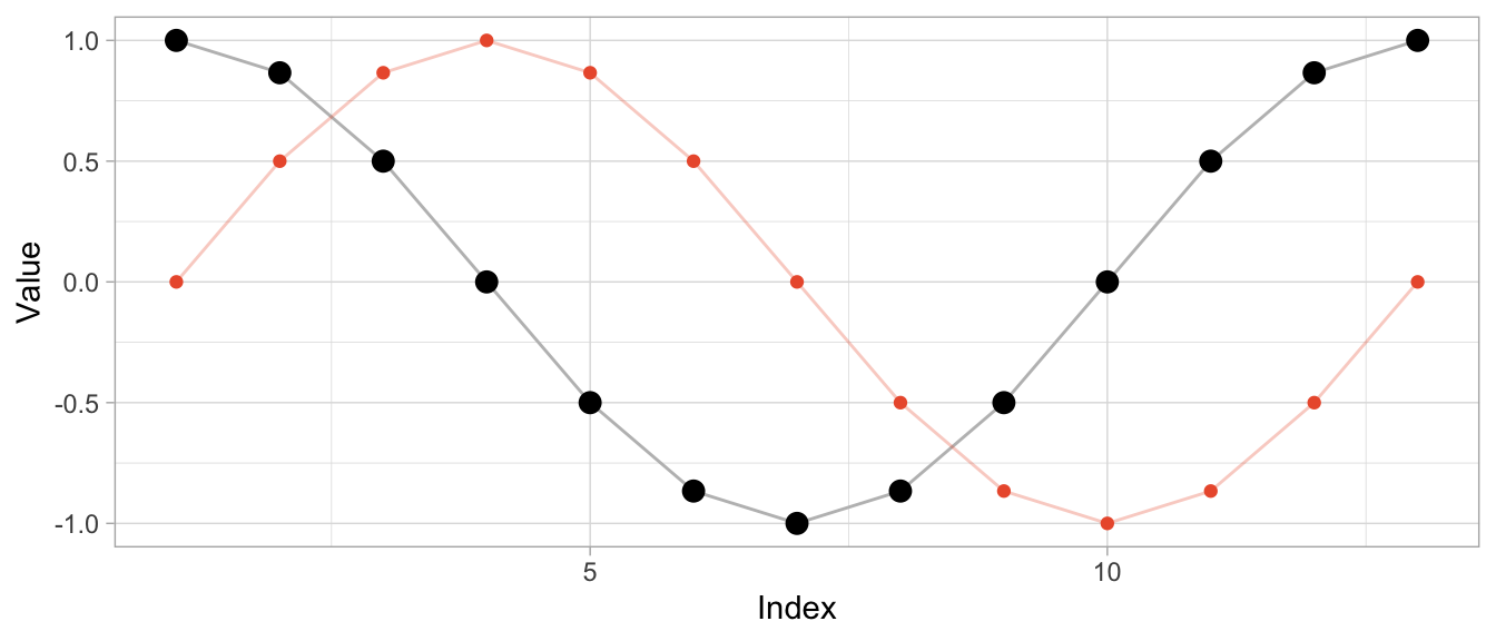
To compute the aligned versions, I use the DTW implementation of the dtw package (also available for Python as dtw-python) with default parameters.
library(dtw)
dtw_shift <- dtw::dtw(x = series_sine, y = series_cosine)
Besides returning the distance of the aligned series, DTW produces a mapping of original series to aligned series in the form of alignment vectors dtw_shift$index1 and dtw_shift$index2. Using those, I can visualize both the original time series and the aligned time series along with the repetitions used for alignment.
# DTW returns a vector of indices of the original observations
# where some indices are repeated to create aligned time series
dtw_shift$index2
## [1] 1 1 1 1 2 3 4 5 6 7 8 9 10 11 12 13# In this case, the first index is repeated thrice so that the first
# observation appears four times in the aligned time series
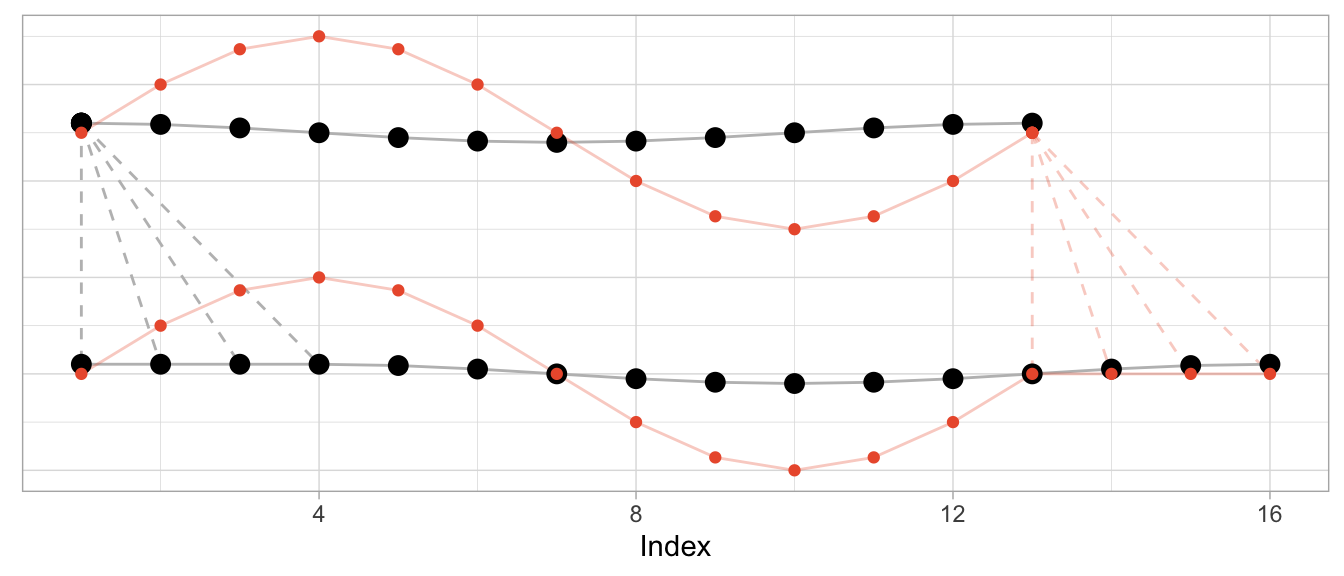
series_cosine[dtw_shift$index2] |> head(8) |> round(2)## [1] 1.00 1.00 1.00 1.00 0.87 0.50 0.00 -0.50The plot below shows the original time series in the upper half and the aligned time series in the lower half, with the sine in orange and the cosine in black. Dashed lines indicate where observations were repeated to achieve the alignment.
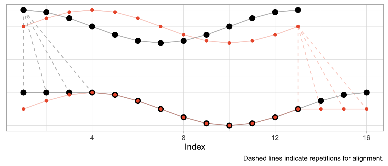
Given that the sine is a perfect shifted copy of the cosine, three-quarters of the observed period can be aligned perfectly. The first quarter of the sine and the last quarter of the cosine’s period, however, can’t be aligned and stand on their own. Their indices are mapped to the repeated observations from the other time series, respectively.
Aligning Speed
Instead of shifting the cosine, I can sample it at a different speed (or, equivalently, observe a cosine of different frequency) to construct a different time series that can be aligned well by DTW. In that case, the required alignment is not so much a shift as it is a squeezing and stretching of the observed series.
Let’s create a version of the original cosine that is twice as “fast”: In the time that we observe one period of the original cosine, we observe two periods of the fast cosine.
series_cosine_fast <- cospi((0:12) / 3)
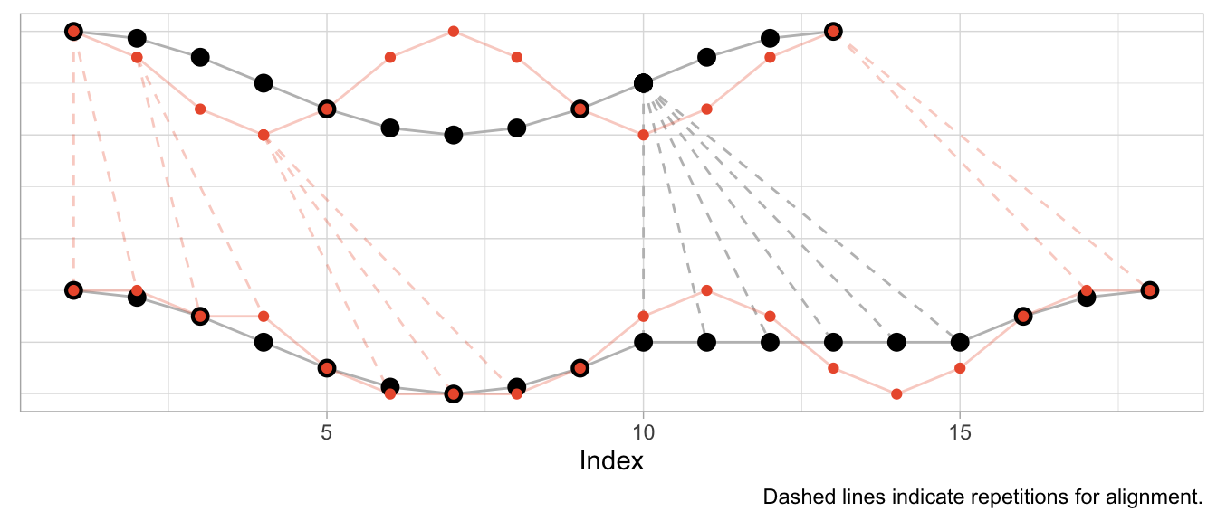
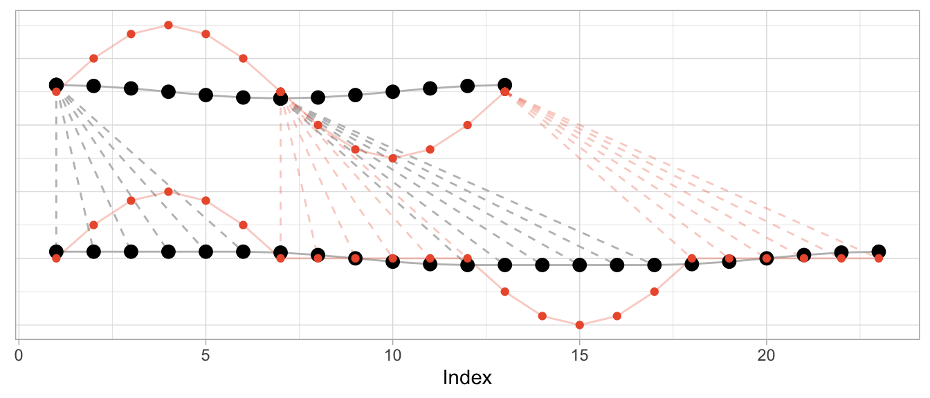
dtw_fast <- dtw::dtw(x = series_cosine_fast, y = series_cosine)The resulting alignment mapping looks quite different than in the first example. Under a shift, most observations still have a one-to-one mapping after alignment. Under varying frequencies, most observations of the faster time series have to be repeated to align. Note how the first half of the fast cosine’s first period can be neatly aligned with the first half of the slow cosine’s period by repeating observations (in an ideal world exactly twice).
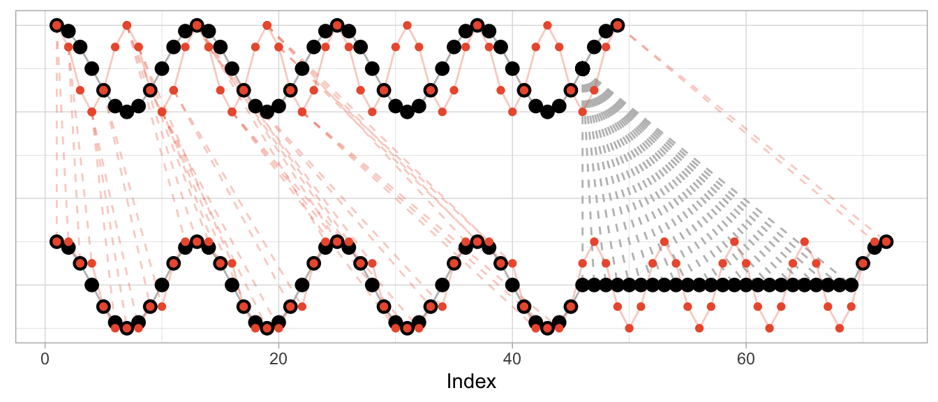
The kind of alignment reveals itself better when the time series are observed for more than just one or two periods. Below, for longer versions of the same series, half of the fast time series can be matched neatly with the slow cosine as we observe twice the number of periods for the fast cosine.
Aligning Different Scales
What’s perhaps unexpected, though, is that the alignment works only on the time dimension. Dynamic time warping will not scale the time series’ amplitude. But at the same time DTW is not scale independent. This can make the alignment fairly awkward when time series have varying scales as DTW exploits the time dimension to reduce the cumulative distance of observations in the value dimension.
To illustrate this, let’s take the sine and cosine from the first example but scale the sine’s amplitude by 5 and check the resulting alignment.
series_sine_scaled <- series_sine * 10
dtw_scaled <- dtw::dtw(x = series_sine_scaled, y = series_cosine)
We might expect DTW to align the two series as it did in the first example above with unscaled series. After all, the series have the same frequencies as before and the same period shift as before.
This is what the alignment would look like using the alignment vectors from the first example above based on un-scaled observations. While it’s a bit hard to see due to the different scales, the observations at peak amplitude are aligned (e.g., indices 4, 10, 16) as are those at the minimum amplitude (indices 7 and 13).
But Dynamic Time Warping’s optimization procedure doesn’t actually try to identify characteristics of time series such as their period length to align them. It warps time series purely to minimize the cumulative distance between aligned observations. This may lead to a result in which also the periodicity is aligned as in the first and second examples above. But that’s more by accident than by design.
This is how DTW actually aligns the scaled sine and the unscaled cosine:
The change in the series’ amplitude leads to a more complicated alignment: Observations at the peak amplitude of the cosine (which has the small amplitude) are repeated many times to reduce the Euclidean distance to the already high amplitude observations of the sine. Reversely, the minimum-amplitude of the sine is repeated many times to reduce the Euclidean distance to the already low amplitude observations of the cosine.
DTW Is Good at Many Things…
Dynamic time warping is great when you’re observing physical phenomena that are naturally shifted in time or at different speeds.
Consider, for example, measurements taken in a medical context such as those of an electrocardiogram (ECG) that measures the electrical signals in a patient’s heart. In this context, it is helpful to align time series to identify similar heart rhythms across patients. The rhythms’ periods could be aligned to check whether one patient has the same issues as another. Even for the same person a DTW can be useful to align measurements taken on different days at different heart rates.
data("aami3a") # ECG data included in `dtw` package
dtw_ecg <- dtw::dtw(
  x = as.numeric(aami3a)[1:2880],
  y = as.numeric(aami3a)[40001:42880]
)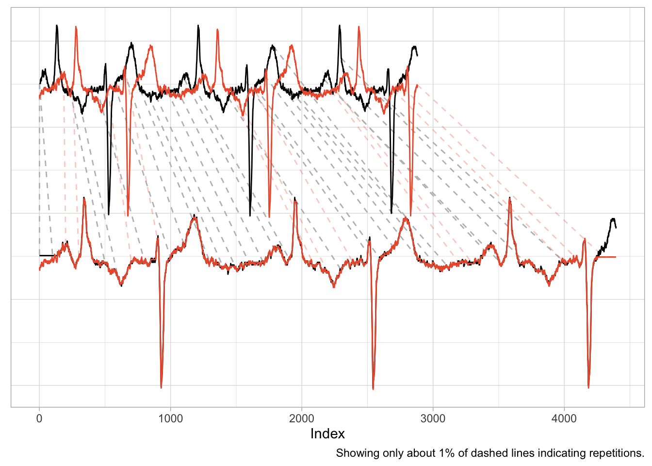
An application such as this one is nearly identical to the first example of the shifted cosine. And as the scale of the time series is naturally the same across the two series, the alignment works well, mapping peaks and valleys with minimal repetitions.
There is also a natural interpretation to the alignment, namely that we are aligning the heart rhythm across measurements. A large distance after alignment would indicate differences in rhythms.
…But Comparing Sales Ain’t One of Them
It is enticing to use Dynamic Time Warping in a business context, too. Not only does it promise a better distance metric to identify time series that are “similar” and to separate them from those that are “different”, but it also has a cool name. Who doesn’t want to warp stuff?
We can, for example, warp time series that count the number of times products are used for patients at a hospital per month. Not exactly product sales but sharing the same characteristics. The data comes with the expsmooth package.
set.seed(47772)
sampled_series <- sample(x = ncol(expsmooth::hospital), size = 2)
product_a <- as.numeric(expsmooth::hospital[,sampled_series[1]])
product_b <- as.numeric(expsmooth::hospital[,sampled_series[2]])
While product_b is used about twice as often as product_a, both products exhibit an increase in their level at around index 40 which is perhaps one characteristic that makes them similar or at least more similar compared to a series that doesn’t share this increase.
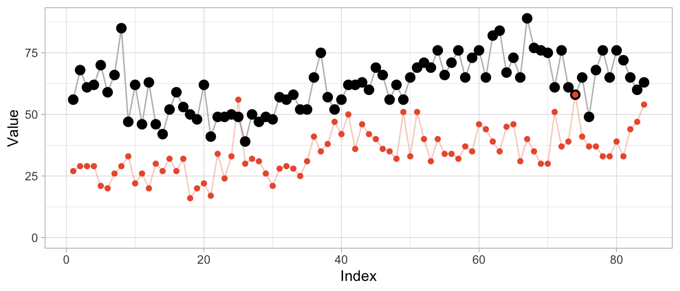
However, the warped versions exhibit a lot of unwanted repetitions of observations. Given the different level of the products, this should not come as a surprise.
dtw_products_ab <- dtw::dtw(x = product_b, y = product_a)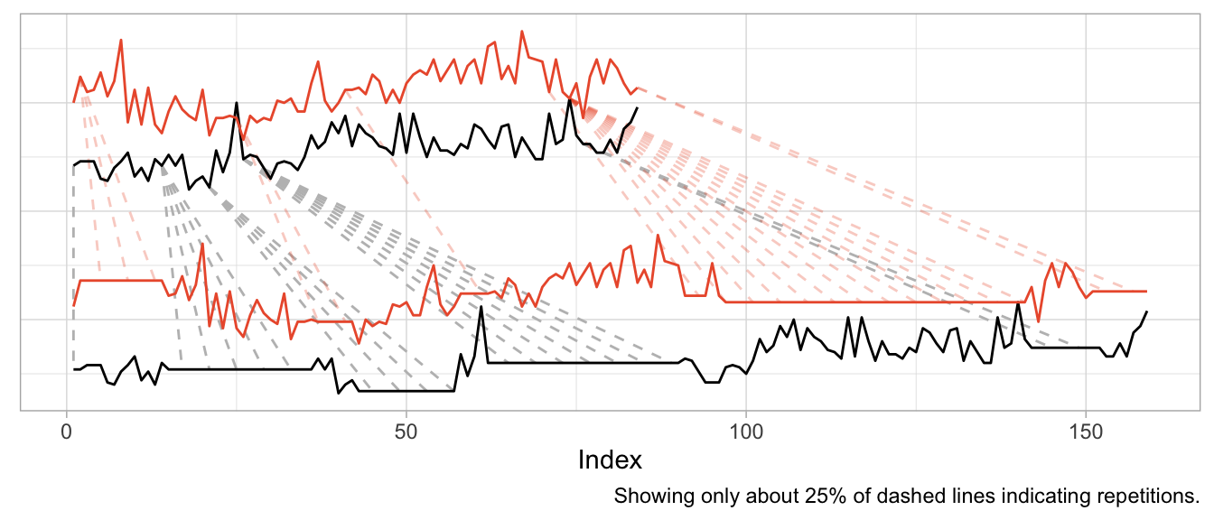
We can mostly fix this by min-max scaling the series, forcing their observations onto the same range of values.
dtw_products_ab_standardized <- dtw::dtw(
  x = (product_b - min(product_b)) / (max(product_b) - min(product_b)),
  y = (product_a - min(product_a)) / (max(product_a) - min(product_a))
)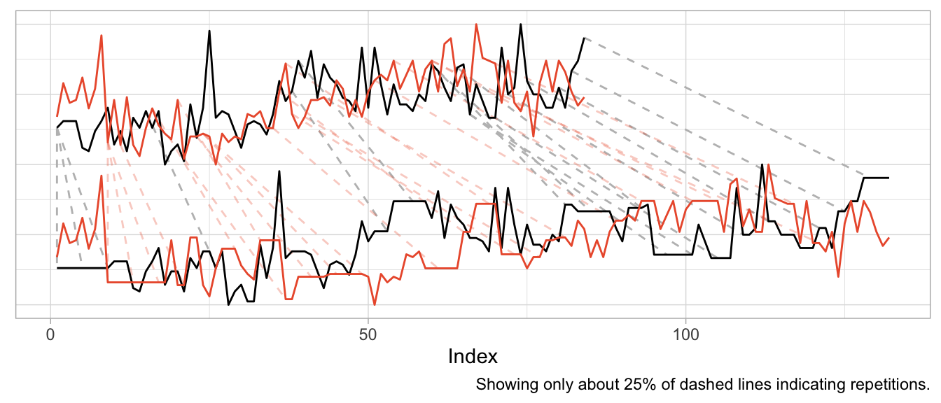
While we got rid of the unwanted warping artifacts in the form of extremely long repetitions of the same observation, the previous plot should raise some questions:
- How can we interpret the modifications for “improved” alignment?
- Are we aligning just noise?
- What does the warping offer us that we didn’t already have before?
If you ask me, there is no useful interpretation to the alignment modifications, because the time series already were aligned. Business time series are naturally aligned by the point in time at which they are observed.2
We also are not taking measurement of a continuous physical phenomenon that goes up and down like the electric signals in a heart. While you can double the amount of ECG measurements per second, it does not make sense to “double the amount of sales measurements per month”. And while a product can “sell faster” than another, this results in an increased amplitude not an increased frequency (or shortened period lengths).
So if you apply Dynamic Time Warping to business time series, you will mostly be warping random fluctuations with the goal of reducing the cumulative distance just that tiny bit more.
This holds when you use Dynamic Time Warping to derive distances for clustering of business time series, too. You might as well calculate the Euclidean distance3 on the raw time series without warping first. At least then the distance between time series will tell you that they were similar (or different) at the same point in time.
In fact, if you want to cluster business time series (or train any kind of model on them), put your focus on aligning them well in the value dimension by thinking carefully about how you standardize them. That makes all the difference.
Before using Dynamic Time Warping, ask yourself: What kind of similarity are you looking for when comparing time series? Will there be meaning to the alignment that Dynamic Time Warping induces in your time series? And what is it that you can do after warping that you weren’t able to do before?
A similar example is also used by the
dtwpackage in its documentation.↩︎Two exceptions come to mind: First, you may want to align time series of products by the first point in time at which the product was sold. But that’s straightforward without DTW. Second, you may want to align products that actually exhibit a shift in their seasonality—such as when a product is heavily affected by the seasons and sold in both the northern and southern hemisphere. DTW might be useful for this, but there might also be easier ways to accomplish it.↩︎
Or Manhattan distance, or any other distance.↩︎