Comes with Anomaly Detection Included

A powerful pattern in forecasting is that of model-based anomaly detection during model training. It exploits the inherently iterative nature of forecasting models and goes something like this:

1. Train your model up to time step t based on data [1,t-1]
2. Predict the forecast distibution at time step t
3. Compare the observed value against the predicted distribution at step t; flag the observation as anomaly if it is in the very tail of the distribution
4. Don’t update the model’s state based on the anomalous observation

For another description of this idea, see, for example, Alexandrov et al. (2019).

Importantly, you use your model to detect anomalies during training and not after training, thereby ensuring its state and forecast distribution are not corrupted by the anomalies.

The beauty of this approach is that

• the forecast distribution can properly reflect the impact of anomalies, and
• you don’t require a separate anomaly detection method with failure modes different from your model’s.

In contrast, standalone anomaly detection approaches would first have to solve the handling of trends and seasonalities themselves, too, before they could begin to detect any anomalous observation. So why not use the model you already trust with predicting your data to identify observations that don’t make sense to it?

This approach can be expensive if your model doesn’t train iteratively over observations in the first place. Many forecasting models¹ do, however, making this a fairly negligiable addition.

But enough introduction, let’s see it in action. First, I construct a simple time series y of monthly observations with yearly seasonality.

set.seed(472)
x <- 1:80
y <- pmax(0, sinpi(x / 6) * 25 + sqrt(x) * 10 + rnorm(n = 80, sd = 10))

# Insert anomalous observations that need to be detected
y[c(55, 56, 70)] <- 3 * y[c(55, 56, 70)]

To illustrate the method, I’m going to use a simple probabilistic variant of the Seasonal Naive method where the forecast distribution is assumed to be Normal with zero mean. Only the \(\sigma\) parameter needs to be fitted, which I do using the standard deviation of the forecast residuals.

The estimation of the \(\sigma\) parameter occurs in lockstep with the detection of anomalies. Let’s first define a data frame that holds the observations and will store a cleaned version of the observations, the fitted \(\sigma\) and detected anomalies…

df <- data.frame(
  y = y,
  y_cleaned = y,
  forecast = NA_real_,
  residual = NA_real_,
  sigma = NA_real_,
  is_anomaly = FALSE
)

… and then let’s loop over the observations.

At each iteration, I first predict the current observation given the past and update the forecast distribution by calculating the standard deviation over all residuals that are available so far, before calculating the latest residual.

If the latest residual is in the tails of the current forecast distribution (i.e., larger than multiples of the standard deviation), the observation is flagged as anomalous.

For time steps with anomalous observations, I update the cleaned time series with the forecasted value (which informs a later forecast at step t+12) and set the residual to missing to keep the anomalous observation from distorting the forecast distribution.

# Loop starts when first prediction from Seasonal Naive is possible
for (t in 13:nrow(df)) {
  df$forecast[t] <- df$y_cleaned[t - 12]
  df$sigma[t] <- sd(df$residual, na.rm = TRUE)
  df$residual[t] <- df$y[t] - df$forecast[t]
  
  if (t > 25) {
    # Collect 12 residuals before starting anomaly detection
    df$is_anomaly[t] <- abs(df$residual[t]) > 3 * df$sigma[t]
  }
  
  if (df$is_anomaly[t]) {
    df$y_cleaned[t] <- df$forecast[t]
    df$residual[t] <- NA_real_
  }
}

Note that I decide to start the anomaly detection not before there are 12 residuals for one full seasonal period, as the \(\sigma\) estimate based on less than a handful of observations can be flaky.

In a plot of the results, the combination of 1-step-ahead prediction and forecast distribution is used to distinguish between expected and anomalous observations, with the decision boundary indicated by the orange ribbon. At time steps where the observed value falls outside the ribbon, the orange line indicates the model prediction that is used to inform the model’s state going forward in place of the anomaly.

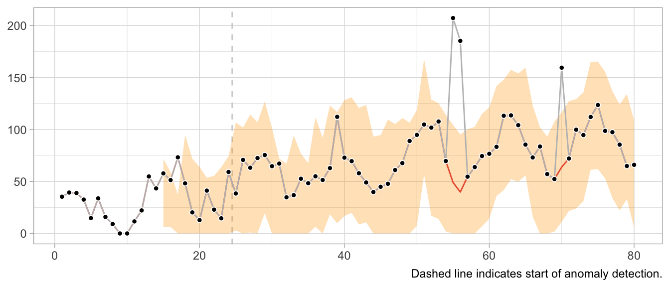
Note how the prediction at time t is not affected by the anomaly at time step t-12. Neither is the forecast distribution estimate.

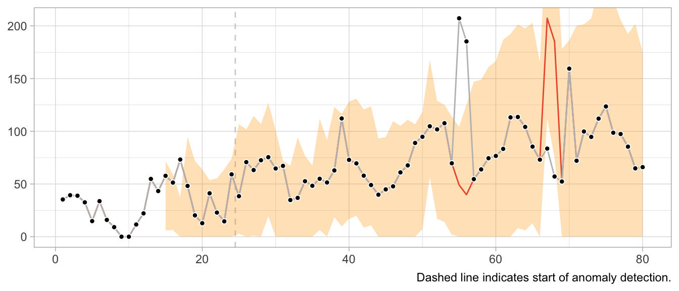
This would look very different when one gets the update behavior slightly wrong. For example, the following implementation of the loop detects the first anomaly in the same way, but uses it to update the model’s state, leading to subsequently poor predictions and false positives, and fails to detect later anomalies.

# Loop starts when first prediction from Seasonal Naive is possible
for (t in 13:nrow(df)) {
  df$forecast[t] <- df$y[t - 12]
  df$sigma[t] <- sd(df$residual, na.rm = TRUE)
  df$residual[t] <- df$y[t] - df$forecast[t]
  
  if (t > 25) {
    # Collect 12 residuals before starting anomaly detection
    df$is_anomaly[t] <- abs(df$residual[t]) > 3 * df$sigma[t]
  }
  
  if (df$is_anomaly[t]) {
    df$y_cleaned[t] <- df$forecast[t]
  }
}