Rediscovering Bayesian Structural Time Series
This article derives the Local-Linear Trend specification of the Bayesian Structural Time Series model family from scratch, implements it in Stan and visualizes its components via tidybayes. To provide context, links to GAMs and the prophet package are highlighted. The code is available here.
I tried to come up with a simple way to detect “outliers” in time series. Nothing special, no anomaly detection via variational auto-encoders, just finding values of low probability in a univariate time series. The week before, I had been toying with generalized additive models (GAMs). So it seemed like a good idea to fit a GAM with a spline-based smooth term to model the trend flexibly while other features take care of everything else (seasonality, …). But really the flexible trend is nice and simple and you don’t even need to think too much:
set.seed(573)

n <- 48
x <- 1:n
y <- rnorm(n, tanh(x / 6 - 4), 0.25 )

gam_fit <- mgcv::gam(y ~ 1 + s(x))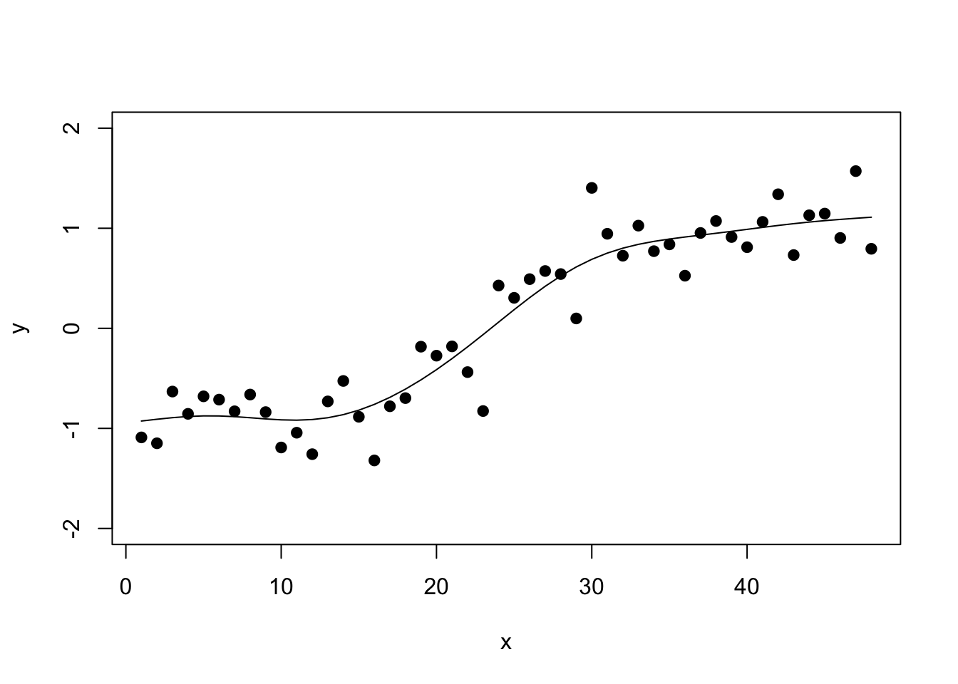
This is all fine and well to get a nice in-sample fit which is all you need for standard outlier detection. For example, the forecast package’s tsoutliers() function relies on the non-parametric stats::supsmu() function to fit a flexible trend.
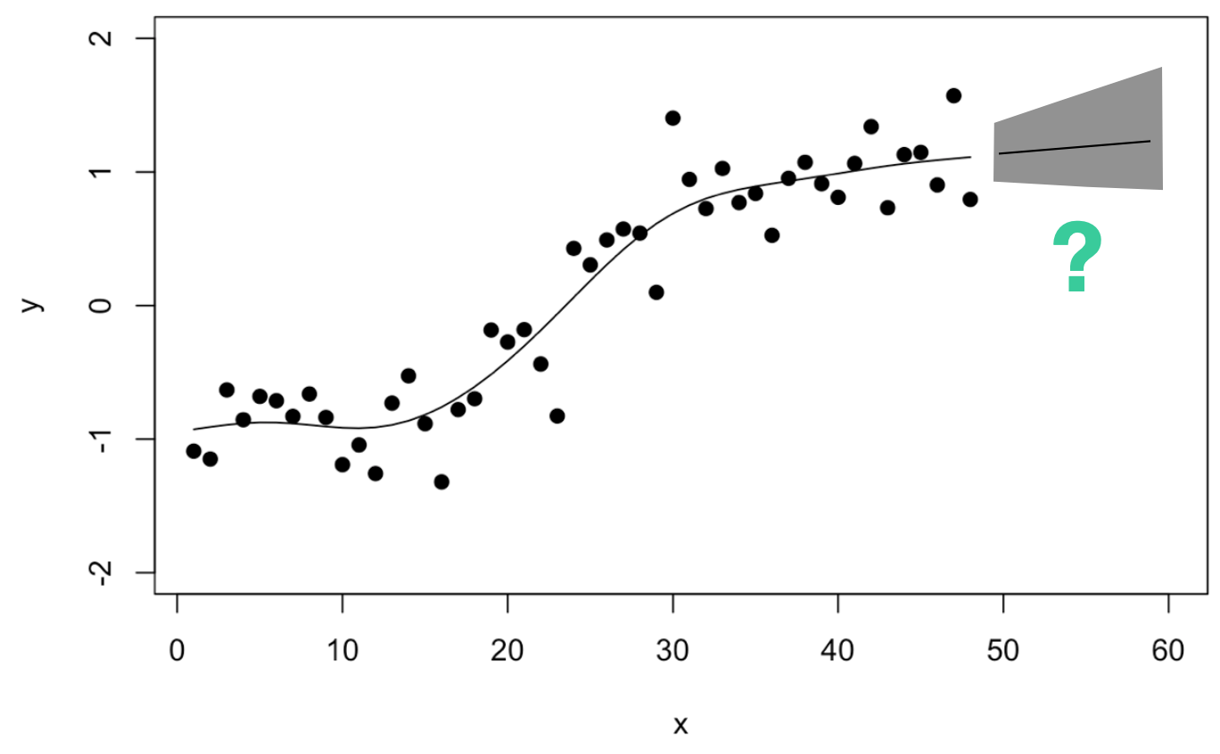
But then I went one step too far: “Wouldn’t it be nice to use a GAM to forecast my time series as well?”
If you’re familiar with spline functions you know this isn’t a question I should have asked myself: When using splines, you are limited to predicting new data that falls into the domain of your training data, i.e. the domain on which the splines were fitted. Once you leave this domain, there are no fitted splines and so your model can’t predict. You can always make assumptions, of course: A linear continuation, using the last value, or similar. But what about your prediction interval?
So I continued thinking: Maybe one could estimate how often the trend has adjusted in the past and use this to derive the prediction interval?
Trend Uncertainty in the prophet Package
In their prophet package, Sean J. Taylor and Benjamin Letham specify their model “similar to a generalized additive model” (Taylor and Letham, 2018) as
\[ y(t) = g(t) + s(t) + h(t) + \epsilon. \]
If we disregard the seasonal \(s(t)\) and holiday components \(h(t)\) for the moment, then this corresponds to the GAM formulation used above. A crucial addition of the prophet package is how Taylor and Letham manage to incorporate uncertainty due to historical trend changes in the model’s prediction intervals (see chapter 3.1 in their paper): In their trend specification,
\[ g(t) = (k + a(t)^T \delta )t + (m+a(t)^T\gamma), \] \(k\) corresponds to the linear growth rate but can be adjusted at changepoints \(a(t)\) by different rate adjustments stored in the vector \(\delta\). In their model specification for Bayesian inference, they pick \(\delta_j \sim \text{Laplace}(0,\tau)\) as prior distribution for the amount by which the rate may change at a changepoint. This implies changes are generally more likely close to zero but can be large from time to time.
It also suggests a convenient approach to forecast the trend uncertainty: They use this generative model to sample new changepoints in the future, as well as new changes in the growth rate via the above prior distribution: Take the estimated rate changes \(\hat{\delta}_j\) and use them to get a maximum likelihood estimate of the Laplace distribution’s scale parameter: \(\hat{\tau} = \frac{1}{S} \sum_{j = 1}^S |\hat{\delta}_j|\).
This provides a way to forecast (the uncertainty of) the piece-wise constant growth rate: Sample new changepoints with linear trend changes according to the distribution fitted to historical growth rate changes.
Could one go a step further and model a continously changing trend as well as its forecast uncertainty? Would this in particular be possible for the spline-based smooth term in the original GAM specified above?
Roughly, this is the direction I went during a late evening whiteboard drawing session:
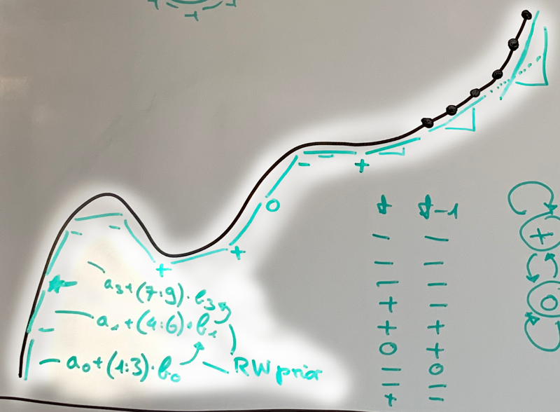
Don’t judge my drawing skills. I believe what I was trying to derive was some sort of local linear approximation to the smooth trend (you see the straight lines for every three observations). Each of the lines would be described by their own coefficients (see \(a_0, b_0, a_1, b_1, ...\) in the lower left corner). And to be fancy, I wrote Random Walk prior to describe how much a coefficient may change from one time point to the next. This is actually not much different from the formulation used in the prophet package: In my drawing, we have a potential changepoint every third observation and instead of changes drawn from a Normal distribution (random walk prior), prophet assumes the Laplace.
A little later that evening it hit me: I already know this! The model I was sketching is equivalent to the local-linear trend Bayesian structural time series model (Scott and Varian 2014)—which itself is equivalent to a dynamic linear model or a state-space model formulation. For the close cousin of the local-level model, look no further than me using it here.
Let’s have a closer look at this model that promises to be sufficiently flexible for many trends, can incorporate other features, is interpretable, and propagates the uncertainty from trend changes into the forecasts.
Bayesian Structural Time Series
We are looking for a flexible way of describing the trend \(\mu_t\) of a time series. Assume that the observations of the time series are the sum of potentially several components: the trend, seasonality, regressors and noise:
\[ Y_t \sim \text{Normal}(\lambda_t, \sigma_Y), \quad \lambda_t = \mu_t + \tau_t + \beta^Tx_t \]
While the seasonal and regressor components are certainly interesting, we’ll focus on the trend for now.
Following my sketch above, what we expect to have is a trend \(\mu_t\) that is a linear function of time, something along the lines of \(\mu_t = \delta_t \cdot t\). This is equivalent to \(\mu_t = \mu_{t-1} + \delta_t\) given that we only consider equal time steps of size 1. So we expect that the trend at the next step is the previous trend plus a smoothly changing difference \(\delta_t\). Adding some additional noise to this relationship, we get
\[ \mu_t = \mu_{t-1} + \delta_t + \epsilon_{\mu,t}, \quad \epsilon_{\mu,t} \sim \text{Normal}(0, \sigma_\mu). \] If the change \(\delta_t\) at each time would be constant at \(\delta\), then the trend would be equal to a linear regression against time. If we let \(\delta_t\) change over time, however, the trend can become a rather flexible function of time—while being locally linear in time.
How do we let \(\delta_t\) change over time? This is where the random walk prior from the whiteboard sketch comes in:
\[ \delta_t = \delta_{t-1} + \epsilon_{\delta,t}, \quad \epsilon_{\delta,t} \sim \text{Normal}(0, \sigma_\delta) \]
Note that this model encompasses a few special cases. First, if \(\delta_t\) was fixed at 0, then the trend \(\mu_t\) would adjust according to a random walk and we would be looking at the local-level model (as used here). Second, if \(\sigma_\delta\) was 0 and thus \(\epsilon_{\delta,t}\) was 0, the trend \(\mu_t\) would be changing according to the linear model—either with some noise or in a straight line if \(\sigma_{\mu}\) was 0.
Generating a Time Series
Given this model, we can generate a time series that follows this model exactly. This provides us with additional intuition with regard to how the different parameters interact.
Here, we generate \(T=40\) observations. We draw \(\sigma_{\mu}, \sigma_{\delta}\) and \(\sigma_Y\) from Half-Normal prior distributions with different scale.
set.seed(4539)

T <- 40
y <- rep(NA, T)

# Draw standard normal errors which will be
# multiplied by the scale later
mu_err <- rnorm(T, 0, 1)
delta_err <- rnorm(T, 0, 1)

s_obs <- abs(rnorm(1, 0, 10))
s_slope <- abs(rnorm(1, 0, 0.5))
s_level <- abs(rnorm(1, 0, 0.5))
## [1] "Scale of Observation Noise: 10.33"## [1] "Scale of Trend Noise: 0.06"## [1] "Scale of Slope Noise: 0.68"Note how the scale of the trend noise is quite small which means that we will not see a strong random walk behavior on the trend.
Also note how we were able to sample the different noise values independently for each time step. We can add them up according to our model by iterating over the time steps. In the final step, we draw the observations from the Normal distribution with mean equal to the trend.
mu <- rep(NA, T)
delta <- rep(NA, T)

mu[1] <- mu_err[1]
delta[1] <- delta_err[1]

for (t in 2:T) {
  mu[t] <- mu[t-1] + delta[t-1] + s_level * mu_err[t]
  delta[t] <- delta[t-1] + s_slope * delta_err[t]
}

y <- rnorm(T, mu, s_obs)
The time series looks as follows:
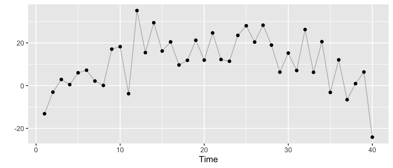
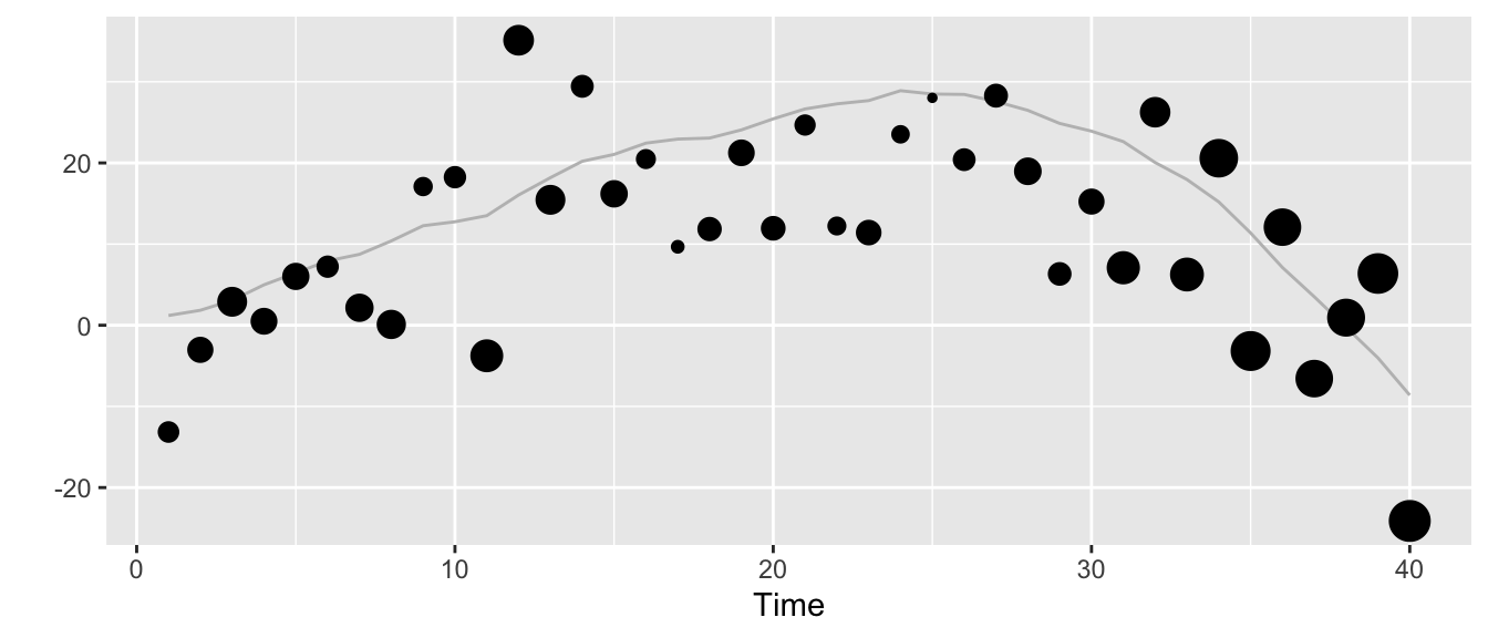
But we can also stylize it differently. The next plot shows the trend \(\mu_t\) as the grey line, the observations \(y_t\) as dots with size scaled according to the size of the change \(\delta_t\) in trend at time \(t\).
Estimating the Model
While there may be more efficient inference methods for this model (Kalman filter) and the ready-to-use bsts package, we can take the specification above to define a Stan model and run Bayesian inference via Hamiltonian Monte-Carlo.
A simple implementation of the local-linear trend model in Stan code looks quite similar to the R code we used to generate the example time series:
library(rstan)
rstan_options(auto_write = TRUE)
options(mc.cores = parallel::detectCores())

llt_model <- stan_model("local_linear_trend.stan",
                        model_name = "local_linear_trend")
## S4 class stanmodel 'local_linear_trend' coded as follows:
## // https://discourse.mc-stan.org/t/bayesian-structural-time-series-modeling/2256/2
##
## data {
## int <lower=0> T;
## vector[T] y;
## }
## parameters {
## vector[T] mu_err;
## vector[T] delta_err;
## real <lower=0> s_obs;
## real <lower=0> s_slope;
## real <lower=0> s_level;
## }
## transformed parameters {
## vector[T] mu;
## vector[T] delta;
## mu[1] = mu_err[1];
## delta[1] = delta_err[1];
## for (t in 2:T) {
## mu[t] = mu[t-1] + delta[t-1] + s_level * mu_err[t];
## delta[t] = delta[t-1] + s_slope * delta_err[t];
## }
## }
## model {
## s_obs ~ normal(5,10);
## s_slope ~ normal(0,1);
## s_level ~ normal(0,1);
##
## mu_err ~ normal(0,1);
## delta_err ~ normal(0,1);
##
## y ~ normal(mu, s_obs);
## }In the next step, we fit the model to the data generated above.
llt_fit <- sampling(object = llt_model,
                    data = list(T = T, y = y),
                    chains = 4,
                    iter = 4000,
                    seed = 357,
                    verbose = TRUE,
                    control = list(adapt_delta = 0.95))
For the three scale parameters, we get the following summary statistics of the samples from their posterior distributions:
print(llt_fit, pars = c("s_obs", "s_level", "s_slope"))## Inference for Stan model: local_linear_trend.
## 4 chains, each with iter=4000; warmup=2000; thin=1;
## post-warmup draws per chain=2000, total post-warmup draws=8000.
##
## mean se_mean sd 2.5% 25% 50% 75% 97.5% n_eff Rhat
## s_obs 9.20 0.01 1.13 7.27 8.41 9.10 9.89 11.64 7350 1
## s_level 0.74 0.01 0.57 0.03 0.29 0.63 1.06 2.12 6384 1
## s_slope 0.67 0.00 0.30 0.24 0.45 0.62 0.83 1.37 3830 1
##
## Samples were drawn using NUTS(diag_e) at Fri May 8 20:42:10 2020.
## For each parameter, n_eff is a crude measure of effective sample size,
## and Rhat is the potential scale reduction factor on split chains (at
## convergence, Rhat=1).Visualizing the Fitted Model
We can use the excellent tidybayes model by Matthew Kay to visualize the fitted model. First off, let’s look at the posterior distributions for the scale parameters for each of the four Markov chains:
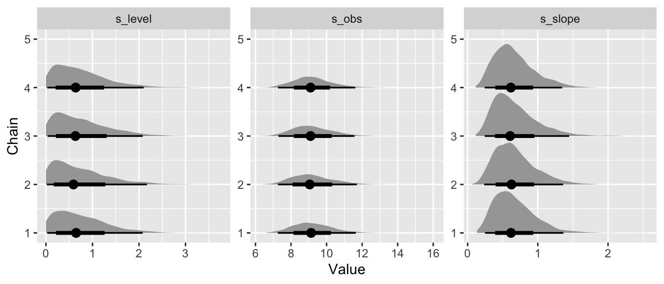
While this is nice, wait until you see the following.
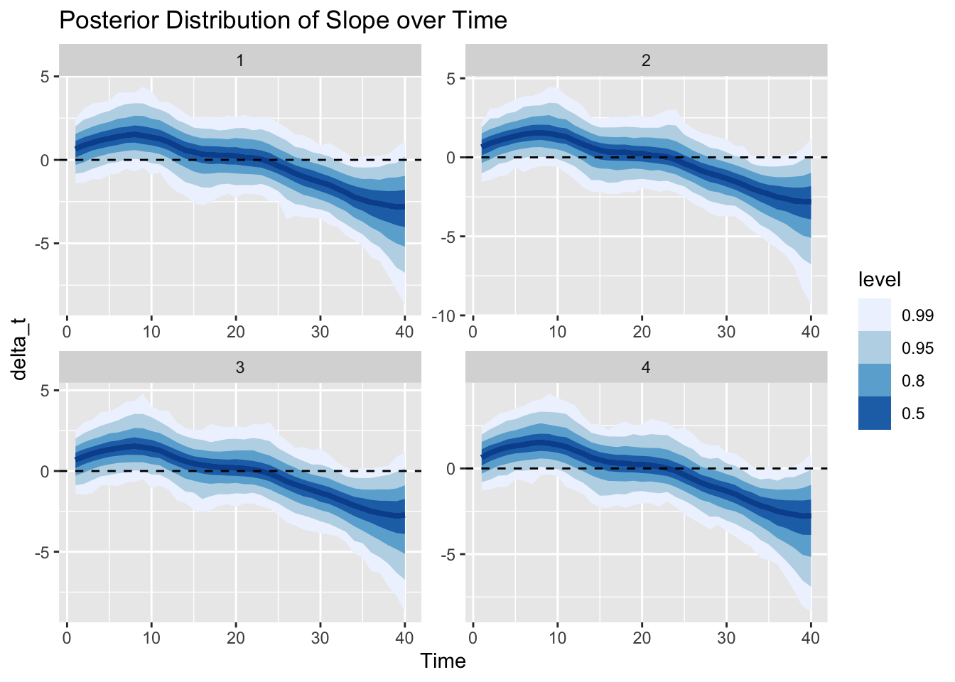
We can visualize the estimated posterior distributions of the slope of the trend, \(\delta_t\), over time. Larger values in absolute terms correspond to period where the overall level of the time series will change more rapidly, while positive values correspond to periods of increasing trend and a negative slope corresponds to periods of decreasing trend.
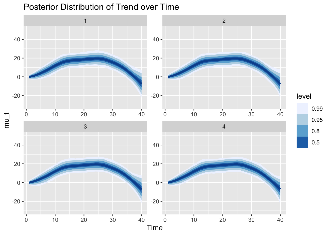
In just the same way, we can also visualize the posterior distribution of the trend \(\mu_t\) over time. The trend increases as the slope above has positive values, then becomes constant as the slope hovers around 0, and changes to decreasing as the slope drops below 0.
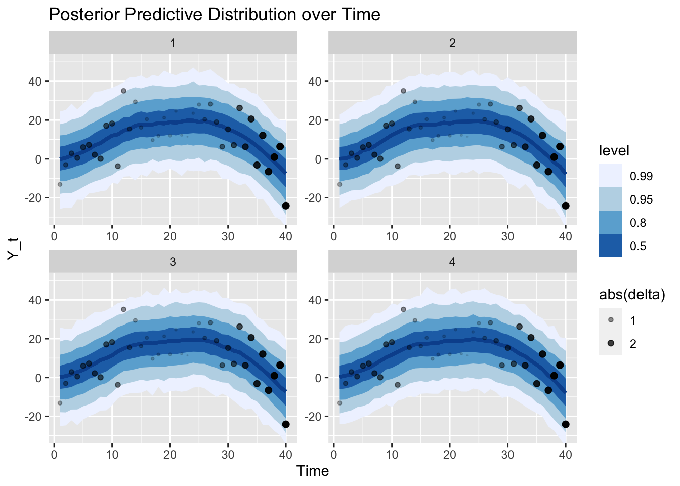
Given the posterior of the trend, we can also sample from our model (i.e., our data generating process) to get samples from the posterior predictive distribution. That is, we now look at the uncertainty of the observations instead of parameters. Note that the y-axis has the same scale as in the graph of the trend before. The different scale of the uncertainty is the result of the additional observation noise \(\epsilon_{Y,t}\). We can say, for example, that the trend is larger than 0 with probability larger than 99% at time step 20. However, observations are still expected to be below 0 with about 10%.
Additionally, we plot the actual observations again with size according to the median of \(\delta_t\)’s posterior distribution.
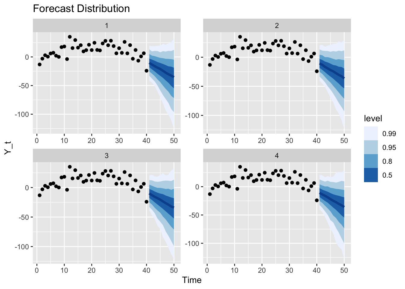
Finally, we can generate and graph the forecast of the time series from the estimated model for the next 10 time steps. Note that all the uncertainty from the parameters’ posterior distributions has been propagated into this forecast distribution.
We can generate new observations that continue the original time series according to the random sampling scheme above and compare against the forecast:
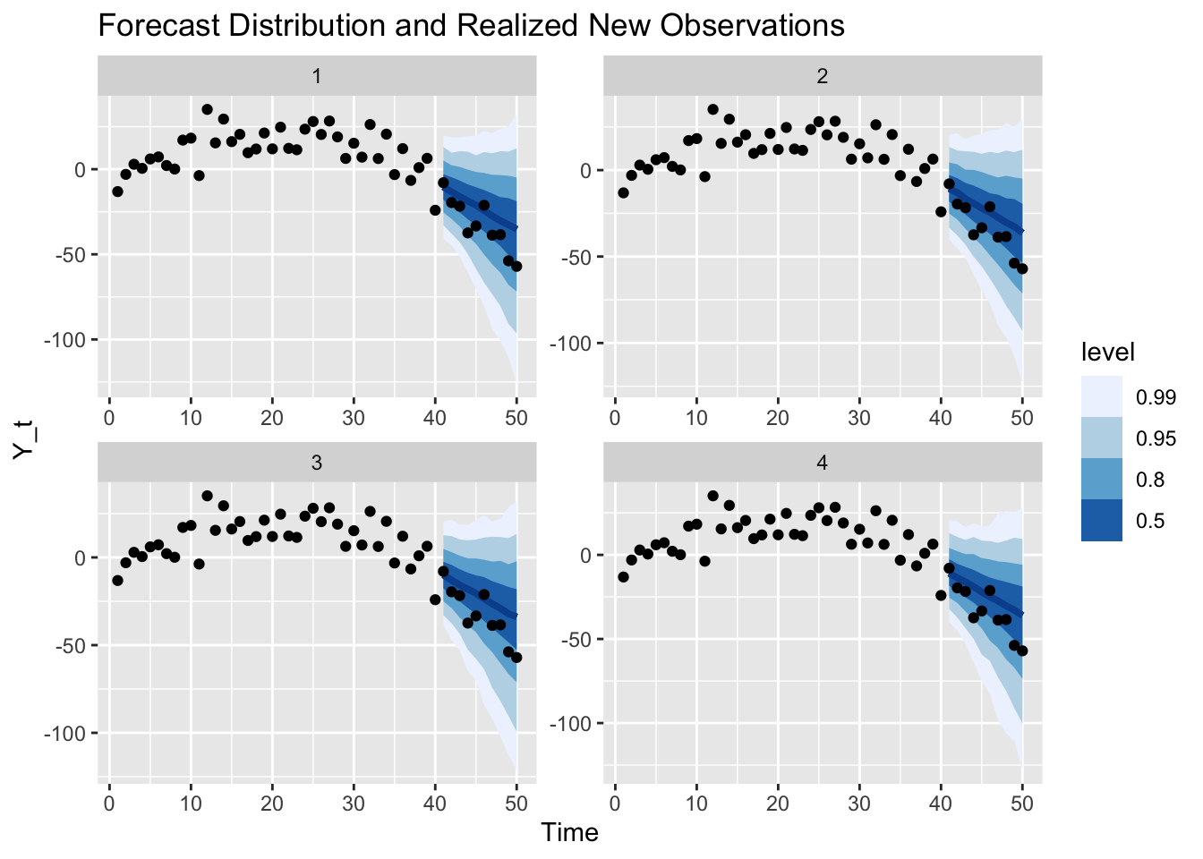
These realized values are of course only one of many possible future outcomes: Had I chosen a different seed, we would have sampled different observations from the same model.
To illustrate the point that there are many different legitimate future outcomes, we can sample paths from our model and visualize those instead of the intervals.
Where to Go From Here
So far I’ve only touched the surface of what’s possible with (Bayesian) structural time series models. But the derivation above has helped me to really come to grips with the idea and sold me on this way of phrasing the time series problem. As described in the information on Andrew Harvey’s book on the topic:
Unlike the traditional ARIMA models, structural time series models consist explicitly of unobserved components, such as trends and seasonals, which have a direct interpretation.
Building on these first steps, we can go further. We could, for example, make use of the interpretability of this model family to automatically provide explanations of the estimated models and their forecasts. This might support conversations with stakeholders.
Another favorite of mine are prior-predictive checks. Combined with Bayesian structural time series models, we would check for a given specification of model and prior distributions which kind of time series that model generates—similar to how we generated a single time series above. Based on this we could adjust the prior distributions to build models that correspond to our prior belief.
An obvious next step would be the implementation of further variants of structural time series models: For example, models with different trend specifications, models that include seasonal components, or with distributions different from the Normal distribution used above. The bsts package and Steven L. Scott’s blog post on the topic are a great place to start on this.
Lastly, the code to reproduce the examples above is available on Github.
References
Steven L. Scott and Hal R. Varian (2014). Predicting the present with Bayesian structural time series. International Journal of Mathematical Modelling and Numerical Optimisation, vol. 5 (2014), pp. 4-23, https://research.google/pubs/pub41335.
Kim Larsen (2016). Sorry ARIMA, but I’m Going Bayesian. Stitch Fix MultiThreaded blog, https://multithreaded.stitchfix.com/blog/2016/04/21/forget-arima/.
Steven L. Scott (2017). Fitting Bayesian Structural Time Series with the bsts R Package. The Unofficial Google Data Science blog, http://www.unofficialgoogledatascience.com/2017/07/fitting-bayesian-structural-time-series.html.
Sean J. Taylor and Benjamin Letham (2018). Forecasting at Scale, The American Statistician 72(1):37-45, https://peerj.com/preprints/3190.pdf.
Andrew C. Harvey (1990). Forecasting, Structural Time Series Models and the Kalman Filter. Cambridge University Press, https://doi.org/10.1017/CBO9781107049994.
Bob Carpenter, Andrew Gelman, Matthew D. Hoffman, Daniel Lee, Ben Goodrich, Michael Betancourt, Marcus Brubaker, Jiqiang Guo, Peter Li, and Allen Riddell (2017). Stan: A probabilistic programming language. Journal of Statistical Software 76(1). doi: 10.18637/jss.v076.i01.
Stan Development Team (2018). RStan: the R interface to Stan. R package version 2.17.3. http://mc-stan.org.
Matthew Kay (2020). tidybayes: Tidy Data and Geoms for Bayesian Models. doi: 10.5281/zenodo.1308151, R package version 2.0.3.9000, http://mjskay.github.io/tidybayes/.
Steven L. Scott (2020). bsts: Bayesian Structural Time Series, R Package version 0.9.5, https://cran.r-project.org/web/packages/bsts/index.html.
Giovanni Petris (2020). dlm: Bayesian and Likelihood Analysis of Dynamic Linear Models, R Package version 1.1-5, https://cran.r-project.org/web/packages/dlm/index.html.
Stan Prior Choice Recommendations. https://github.com/stan-dev/stan/wiki/Prior-Choice-Recommendations.
Notes by Ben Goodrich on implementing latent time series models in Stan on the Stan Discourse. https://discourse.mc-stan.org/t/bayesian-structural-time-series-modeling/2256/2.
Marko Laine (2019). Introduction to Dynamic Linear Models for Time Series Analysis. arXiv Preprint, https://arxiv.org/pdf/1903.11309.pdf.
Tim Radtke (2020). The Causal Effect of New Year’s Resolutions. Minimize Regret blog, https://minimizeregret.com/post/2020/01/18/the-causal-effect-of-new-years-resolutions/.