The Causal Effect of New Year’s Resolutions
We treat the turn of the year as an intervention to infer the causal effect of New Year’s resolutions on McFit’s Google Trend index. By comparing the observed values from the treatment period against predicted values from a counterfactual model, we are able to derive the overall lift induced by the intervention.
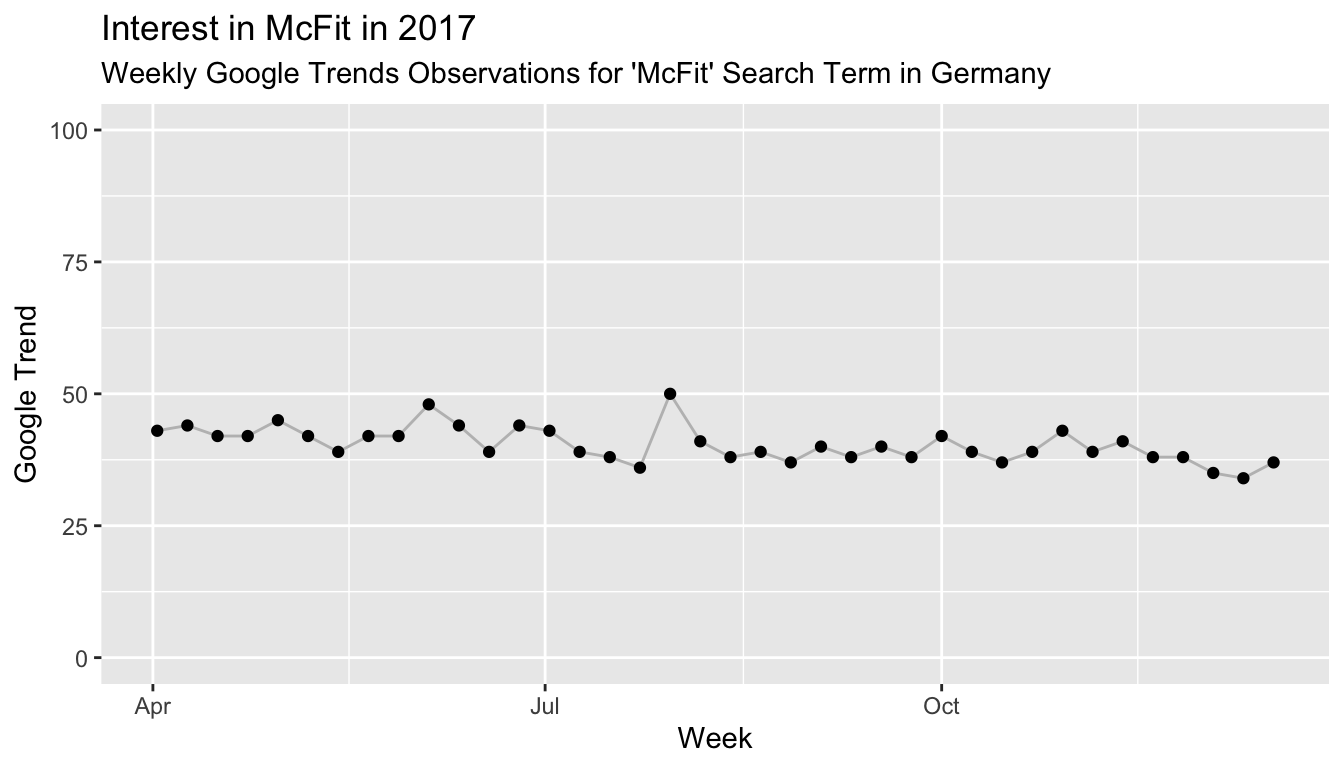
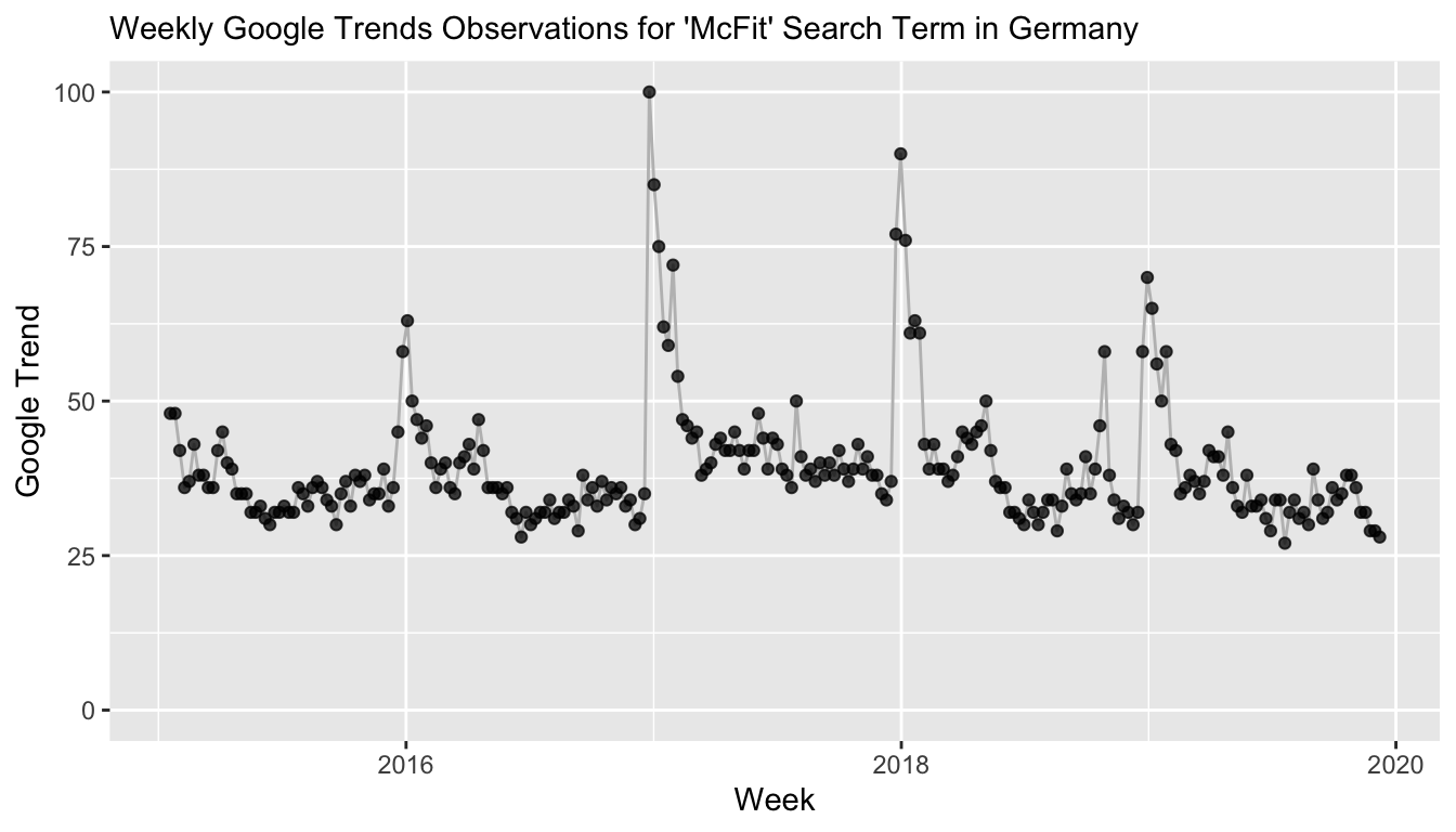
Throughout the year, people’s interest in a McFit gym membership appears quite stable.1 The following graph shows the Google Trend for the search term “McFit” in Germany for April 2017 to until the week of December 17, 2017. Fluctuating somewhere around 40, the “McFit” search term is right in the middle of the 0 to 100 scale used for Google Trends.
But as in many other countries, joining a gym is a typical New Year’s resolution in Germany. So we would expect to observe a jump in interest around the turn of the year, as people promise themselves to add a habit to their lives and to burn the calories they consumed during the holidays.
To estimate the effect that New Year’s resolutions have on the interest in McFit, we will consider the turn of the year as an intervention. The intervention is followed by a period which we will call treatment period. Since we observe a “treated” environment, we would expect to observe different behavior than in the “untreated” region before the intervention and thus a change in the Google Trend index. To estimate the change induced by the treatment, we not only need the actual observations from the treatment period, but also the counterfactual: What would we expect to happen in the absence of the intervention posed by New Year’s? Given that the time series appears to be reasonably forecast-able, a simple approach might be to take this time series’ forecast as counterfactual. This approach and the discussion here is motivated by the paper Inferring causal impact using Bayesian structural time-series models by Brodersen et al. from 2015.
To derive the counterfactual forecast, we thus fit a Bayesian structural time series model—in this case we might use a local level model, in which the observations are generated by a Normal distribution with a mean that changes according to a random walk:2
\[ Y_t \sim N(\mu_t, \sigma) \] \[ \mu_{t+1} \sim N(\mu_t, \tau) \]
Before we use this model to generate a counterfactual on which we base our causal effect inferences, we should ensure that we can actually rely on the model’s prediction.
Evaluation of Forecast Model in Untreated Period
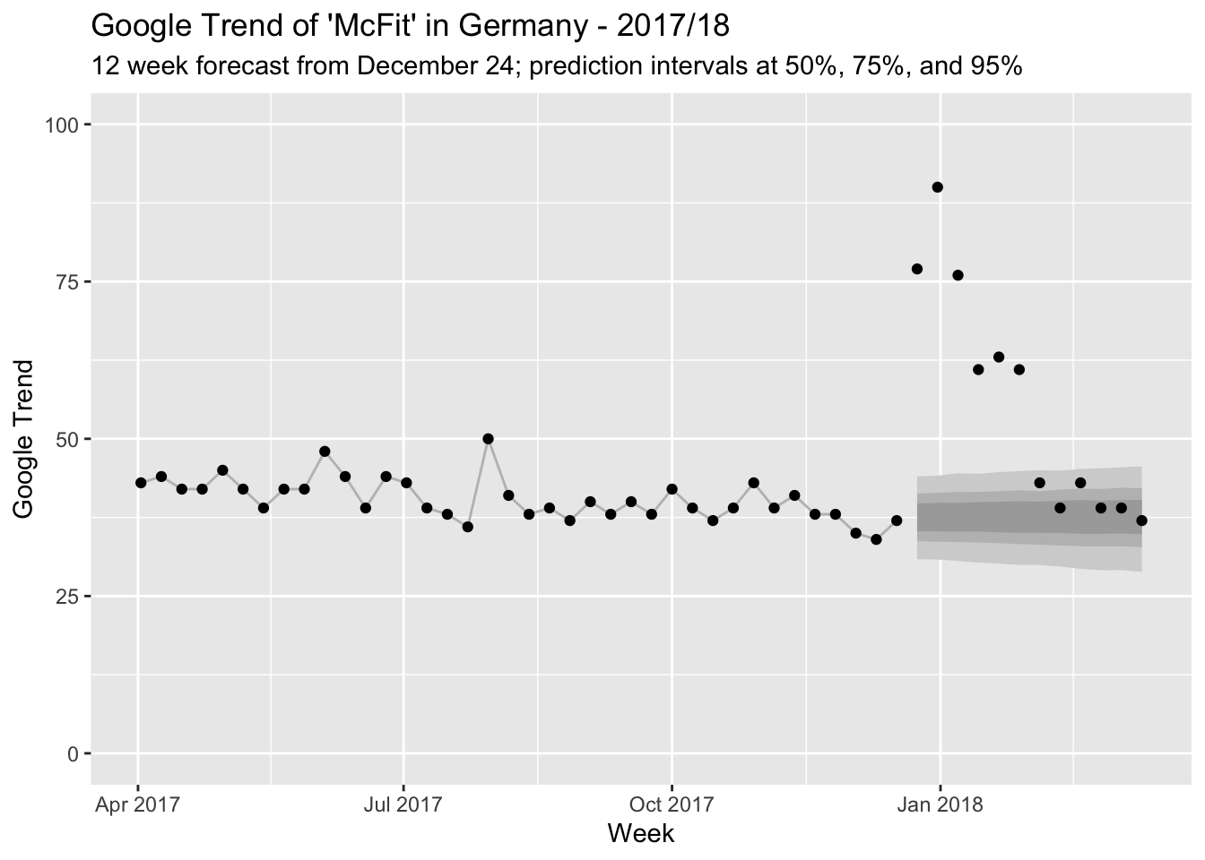
How well can this simple model predict the time series up to this point? To evaluate this, we train it on the first 26 observations in our time series and predict the remaining 12 from October until right before the actual intervention near the end of December. We can fit the above model quickly using the bsts package in R:
range(mcfit_2017_short$week)## [1] "2017-04-02" "2017-09-24"library(bsts)
state_spec_short <- AddLocalLevel(list(), y = mcfit_2017_short$trend)
model_short <- bsts(mcfit_2017_short$trend,
state.specification = state_spec_short,
niter = 11000, ping = 0)pred_short <- predict(model_short, horizon = 12, burn = 1000)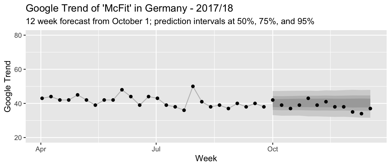
Given how fairly well the prediction intervals describe the actual observations (and since this here is just a blog post), we can be quite confident in the model’s predictions going forward.3
Causal Effect of a Hypothetical Intervention
Since we already have a forecast for the untreated region, we can use this forecast, too, as counterfactual: We can pretend that October 1 also has been an intervention date after which we might observe a treatment effect. Would our model conclude that there has not been any significant change? If it did find a significant change, then this might tell us that our model does not yet account for all behaviors of the time series besides the impact of New Year’s resolutions. In that case, we could not rely on it to provide a accurate counterfactual estimate for our period of interest.
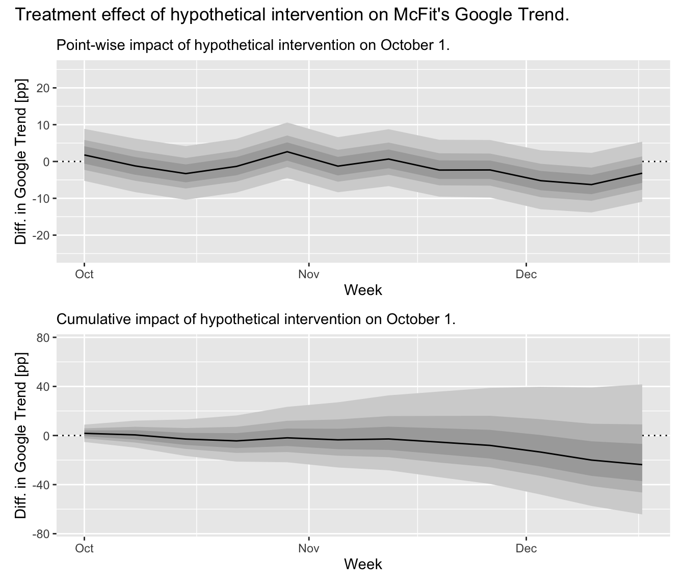
To derive the treatment effect on the untreated region, we subtract the observed trend values from the posterior predictive samples of our forecast model. This provides us not only with a point estimate but the uncertainty in our prediction is propagated as well. Since we are estimating a causal effect on an untreated region, we expect to observe no large evidence for an effect different from zero. Indeed, as the graphs show below, we observe a posterior expectation of a total -20.4 additional Google Trend percentage points over the 12 weeks following October 1. With a 97.5% credible interval at [-64.3, 41.7] percentage points, there is a lot of probability on both sides of zero. This change in percentage points corresponds to an expected lift of -4.4% compared to the counterfactual estimate, with a [-13.9%, 9%] credible interval.
We can thus be fairly confident in using this model to provide a counterfactual estimate when we move to the analysis of the actual intervention around New Year’s.
Causal Effect of Turn-of-the-Year Intervention
With the above analysis in hand, all we need is to take the time series up until the date of the intervention and to re-fit our model. It will provide us with the counterfactual estimate for the treated period. After that, we can observe the actual Google Trend for the treated period and compare against our counterfactual to derive the treatment effect in the same way as we did above.
range(mcfit_2017$week)## [1] "2017-04-02" "2017-12-17"ss <- AddLocalLevel(list(), y = mcfit_2017$trend)
mcfit_model <- bsts(mcfit_2017$trend,
state.specification = ss,
niter = 11000, ping = 0)pred <- predict(mcfit_model, horizon = 12, burn = 1000)The model provides us with the following counterfactual forecast for the beginning of 2018:
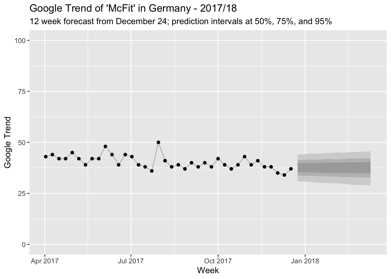
And this is how the counterfactual compares to the observed Google Trend index for McFit:
Wow, people really do like to make New Year’s resolutions! There is probably little discussion about whether something changes after the intervention. But since we have a model at hand, let’s still quantify just how much changes.
To estimate the treatment effect, we proceed as in our dry run above: We subtract the posterior predictive samples from the observed trend values. This let’s us make probabilistic statements about the size of the treatment effect. You can see the result in the graphs below. We observe a posterior expectation of 217.7 additional Google Trend percentage points over the 12 weeks following Christmas. This is a significant effect with a 97.5% credible interval at [165.7, 279] percentage points—far, far away from zero.
What becomes clear from the graph, however, is that this effect is mainly generated within the first 6 weeks after the intervention. After that, the actuals are again somewhat in line with our model (though all lie jointly above the expectation which is an event with somewhat small probability). After 6 weeks, we already have a posterior expectation of 202.8 additional Google Trend percentage points with a 97.5% credible interval at [177.5, 231.6] percentage points. This corresponds to an expected lift of 47.4% compared to the predicted trend, with a [41.5%, 54.1%] credible interval.
In contrast, the pointwise treatment effect estimated in week 12 after the intervention is a difference of -0.5 [-8.6, 8.1] percentage points, corresponding to a tiny lift of -1.4% [-23.3%, 22%] and thus no change compared to the counterfactual scenario.
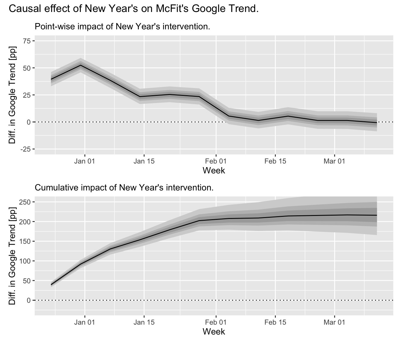
This has shown us that people’s interest in McFit increases suddenly around New Year’s as they make New Year’s resolutions—and that this interest drops rapidly and disappears from February onwards as everyone has either signed up to McFit or lost sight of their resolutions.
Or is there something else in play that could have an effect on people’s behavior?
Causal Effect Entanglement
Alas, the turn of the year is not the only intervention: McFit builds on people’s good intentions with membership fee discounts and marketing campaigns.

A McFit billboard as seen at Berlin walls.
The above image shows a large billboard advertising a McFit membership for only €4.90 per month if you subscribe until January 31, 2020.4 With the slogan “Für mehr wow!” (“For more wow!”), the marketing campaign makes it difficult to understand just how much of the Google Trend peak is caused by the turn of the year—and how much should be attributed to the marketing.5
This is a problem for us since with price discounts and marketing campaigns in place, we can no longer claim confidently that people increasingly search for “McFit” only because of New Year’s resolutions. Instead, the total number of increased searches will have multiple, entangled causes: Some people plan to become fit and think of the McFit brand. Others see a billboard with an enticing offer and want to subscribe online. Again others are comparing gyms to put their New Year’s resolutions in place and search for McFit because they were reminded of it by the marketing campaign. In a sense, New Year’s resolutions are no longer exogenous: They will exist in part because of the contemporaneous McFit marketing, which exists due to New Year’s resolutions and their effect.
Consequently, we cannot conclude which effect is caused by the New Year’s intervention, which by the marketing campaign’s intervention, and which effect by the interaction of the previous two.
What we need is an approach that let’s us disentangle these effects. Surely McFit as a business would be interested in disentangling them to estimate the return on their marketing investment! Maybe all their new customers would have subscribed even without a discount but solely due to their resolutions?
Geographic Experiments
One approach to entangle the effects could be the implementation of a geographic experiment in which certain regions are exposed to a marketing campaign while others are not. For out-of-home and online advertising, this might be feasible, though customers in areas without a campaign could still learn in other ways about the price reduction—and the price reduction potentially has to hold for at least an entire country. McFit, however, is located in multiple countries. If these countries have a similar predisposition for New Year’s resolutions, it might be possible to compare effects across countries by introducing neither price reductions nor marketing campaigns in some of them.
The following papers outline approaches along this line:
- Alberto Abadie, Alexis Diamond, Jens Hainmueller (2009). Synthetic Control Methods for Comparative Case Studies: Estimating the Effect of California’s Tobacco Control Program
- Alberto Abadie (2019). Using Synthetic Controls: Feasibility, Data Requirements, and Methodological Aspects.
- Kay H. Brodersen, Fabian Gallusser, Jim Koehler, Nicolas Remy, Steven L. Scott (2015). Inferring causal impact using Bayesian structural time-series models.
- Jon Waver, Jim Koehler (2011). Measuring Ad Effectiveness Using Geo Experiments.
- Jon Waver, Jim Koehler (2012). Periodic Measurement of Advertising Effectiveness Using Multiple-Test-Period Geo Experiments.
At least the current marketing campaign appears to be active in all countries, though, going from the McFit websites for different countries.
Time-Varying Covariates as Synthetic Controls
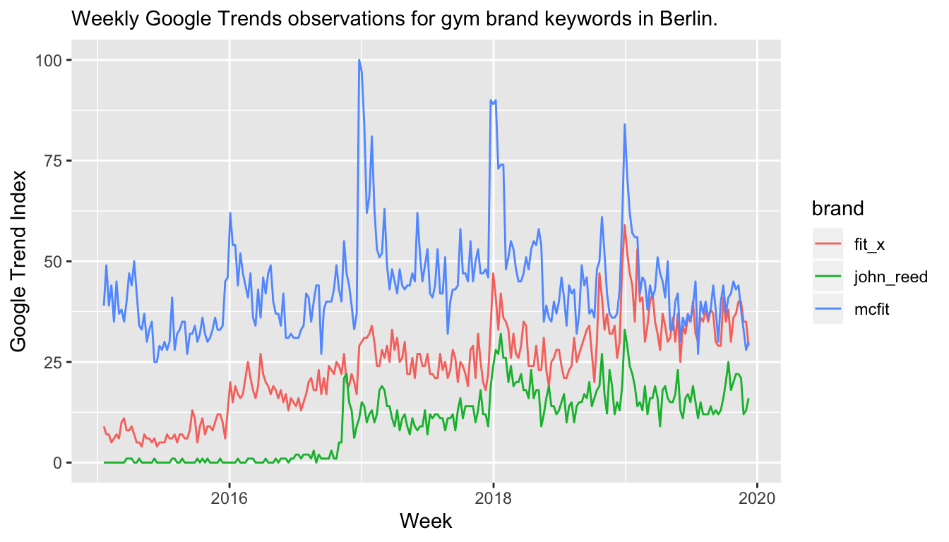
Instead of the simple time series model used above, one could consider including time-varying covariates in the model that are able to predict the behavior of the McFit trend. Since we could train the model before the intervention period, but compute the forecast after the intervention period (when we want to infer the treatment effect based on observed values), we could even use features that are observed at the same time as the McFit trend. For example, one could consider using the Google Trend of other gym brands: We would expect them to have some New Year’s resolutions effect as well. Therefore, their combination could also predict the effect on McFit’s. The difference between the observed Google Trend index and this counterfactual could then be attributed to the fact that a marketing campaign was put in place at the same time (while we could still use the previous model as counterfactual for the new model and infer the impact of resolutions).
This approach has been developed in: Kay H. Brodersen, Fabian Gallusser, Jim Koehler, Nicolas Remy, Steven L. Scott (2015). Inferring causal impact using Bayesian structural time-series models.
The problem with this line of argument is that the Google Trend of other gym brands might or might not be impacted by McFit’s marketing campaign: Before they subscribe to McFit’s offer online, people might have a look at the website of FitX or John Reed.6 If that’s the case, then our covariate-based counterfactual estimate of the trend including the New Year’s resolution effect would be impacted by the treatment effect we try to infer.
In a way, New Year’s resolutions create a similar environment for marketers as Google does with search engine marketing on brand name keywords: Companies pay the “Google tax” to show their SEM advertisement at the top of the search results even though the user was searching for their brand already—just so that other companies don’t attract the user away with their SEM advertisement. Similarly, gym brands could simply take the increased demand due to New Year’s resolutions without even having to advertise. But because someone will advertise, all of them have to create a special offer. Especially when they’re not able to properly estimate the causal impact of their marketing, the situation might end up in a tragedy of the commons (with the increased market demand as common resource).
Forecast Model with Yearly Seasonality
In reality, we have access to more than just one year of data. If we knew that McFit did not run any advertising in the past years around New Year’s, we could estimate a time series model with seasonality in order to properly model the New Year’s resolutions counterfactual effect for the current year—a marketing campaign in the current year would then be evaluated by the difference between the counterfactual forecast and the actuals. In our case however, I would assume that McFit has a marketing campaign every year around New Year’s.
Additionally, we would need to assume that marketing campaigns from other companies are negligiable.
Conclusion
The Google Trend data for McFit offers a natural intervention posed by the turn of the year which provides the opportunity to estimate a causal effect of New Year’s resolutions on human behavior. We observe a large increase in the index that subsequently reverts back to the counterfactual forecast within a few weeks. While we can estimate the effect after the intervention, we can not differentiate between New Year’s resolutions and the change due to a contemporaneous marketing campaign.
Causal inference is hard, even when the observed effects are huge.
The original data is available on Google Trends for the German “McFit” index and for the comparison of three gym brands in Berlin.
For those unfamiliar with German gym brands, according to Wikipedia, “[t]he McFIT GmbH is the largest fitness center chain in Germany”.↩
Note that this corresponds to an Exponential Smoothing model as long as \(\sigma > 0\) and \(\tau > 0\). See this blog post by Steven L. Scott.↩
Note that the last three observations from December show a bit of a dip potentially due to the Advent season. This could be accounted for if we used data from several years to account for seasonality. However, due to the way we consider the data for causal estimation, we act as if there is only this year—else we would know about last year’s New Year effect, too.↩
Of course, the reduced fee applies for the first 6 months after which the contract continues with a fee of at least €19.90 for another 14 months.↩
Note that I actually don’t know whether there has been a marketing campaign in 2017/18, but let’s just assume that there has been.↩
John Reed being owned by the same group as McFit.↩