A Flexible Model Family of Simple Forecast Methods
Introducing a flexible model family that interpolates between simple forecast methods to produce interpretable probabilistic forecasts of seasonal data by weighting past observations.
In business forecasting applications for operational decisions, simple approaches are hard-to-beat and provide robust expectations that can be relied upon for short- to medium-term decisions. They’re often better at recovering from structural breaks or modeling seasonal peaks than more complicated models, and they don’t overfit unrealistic trends.
If that wasn’t enough, they’re interpretable. Not just explainable, but interpretable.
Still, when faced with thousands or millions of time series, not all of them will be modeled best by the naive method, nor will all be modeled best by the seasonal mean. You’d still like to pick a method that fits the series. Similarly, the all-or-nothing nature of approaches such as the seasonal naive method can be a bit black-or-white. A bit more smoothness and impact from multiple past observations can be helpful as long as we don’t compromise in robustness.
Assigning Weights Over Time
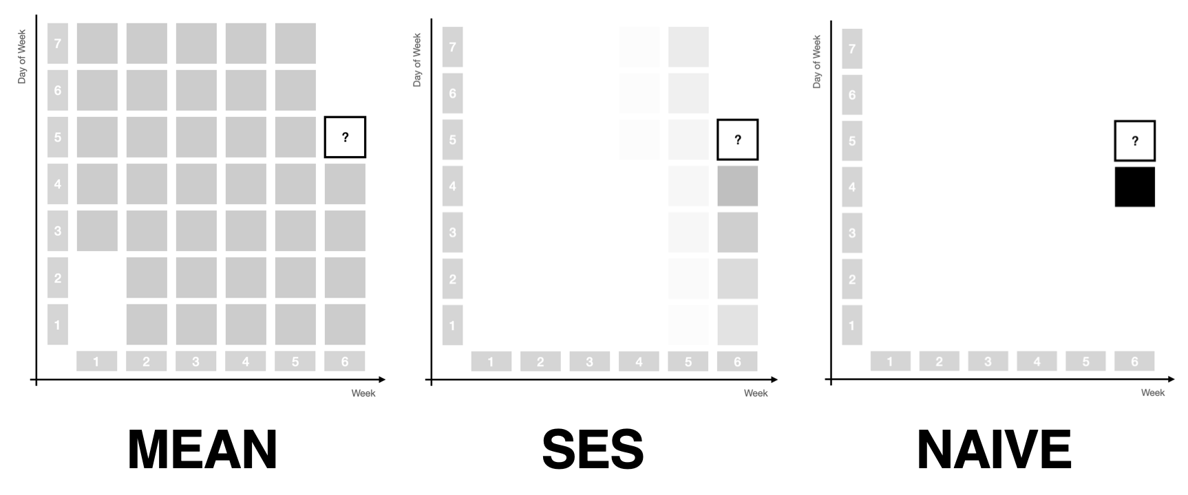
A bit more smoothness is what simple exponential smoothing offers for the mean and naive forecast methods: As you vary the single \(\alpha\) parameter between 0 and 1, simple exponential smoothing will move from the mean forecast to the naive forecast, in between assigning exponentially decreasing weights to past observations. The prediction becomes the weighted average of the past observations. The mean forecast uses the same weight for all observations, whereas the naive method assigns all weight to the most recent observation.
In many applications, however, using only simple exponential smoothing could never suffice. A seasonal component in monthly or daily data is often the main signal that needs to be modeled and projected into the future. Not only are more recent observations more representative of the future, but so are observations that are close in the seasonal period: October 2023 is going to be more similar to September 2022 than to May 2023. Wednesday is more similar to Wednesday last week than to Monday.
This motivates two more ways of weighting past observations.
Assigning Weights Within and Across Seasonal Periods
First, observations can be weighted within a seasonal period. Due to seasonality, the observation exactly a year ago or exactly a week ago should get a larger weight than the observation 11 months ago or two days ago.
Second, observations can be weighted across seasonal periods, assigning more weight to the most recent period than to the period before that and the one before that.
As before, exponential weights make for a useful weighting structure. When assigning weights within a period, each period gets the same weight. When assigning weights across periods, each observation within a period gets the same weight.
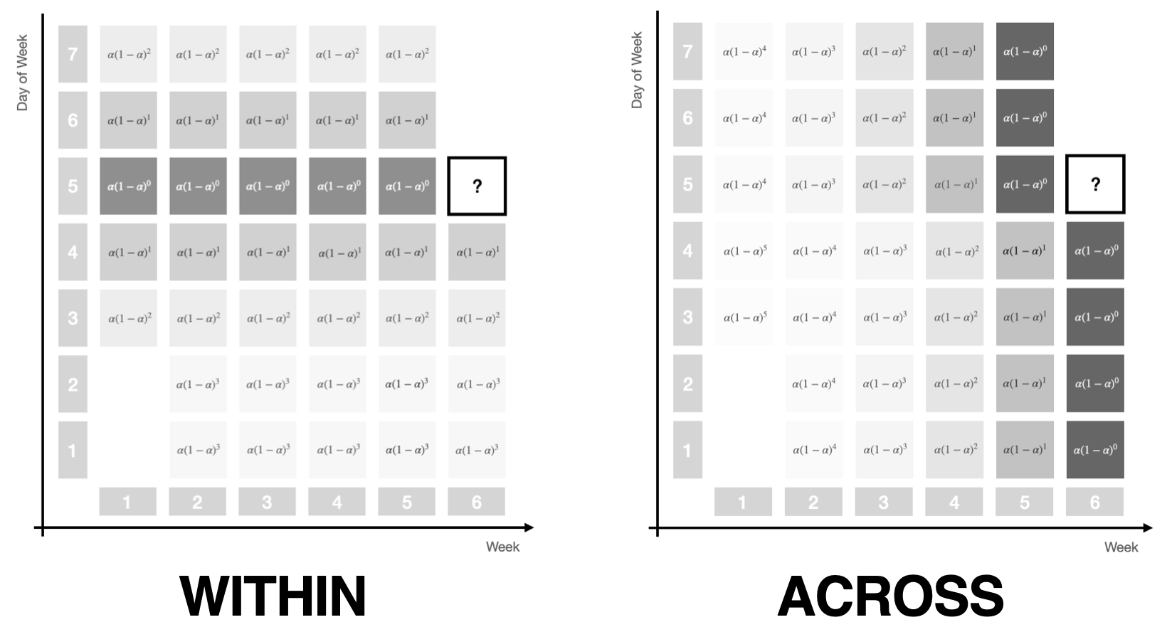
Note how both the within and the across period weighting schemes are each controlled by a single parameter if we give them a similar functional form as used in simple exponential smoothing. The picture above illustrates this by using the familiar \(\alpha (1 - \alpha)^t\) notation.
As we vary the parameter from 0 to 1 for within-period weights, the same weight will be assigned to all observations in the period, then shifts away from observations that are currently in the middle of the period towards the edges, until all weight is assigned to the observation that’s in the same step of the period as the future observation.
For across-period weights, at first the same weight will be assigned to all periods, to then be exponentially decreased for past periods, until all weight will be assigned to just the most recent period.
Assigning Weights Over Time and Seasonal Periods
At this point we have three ways of assigning weights to past observations to move smoothly between forecast methods, namely using
- exponential weights that decrease over time controlled by a parameter \(\alpha\)
- seasonal within-period exponential weights controlled by a parameter \(\alpha_s\), and
- seasonal across-period exponential weights controlled by a parameter \(\alpha_{sd}\).
Combining all three weighting schemes through multiplication1 provides a powerful weight structure that depends on only three parameters and captures most signal sources in time series of operational business applications.
The picture below illustrates the complex weight pattern that this combination can achieve, smoothly assigning weights to observations close in season and time, and then decreasing from there.
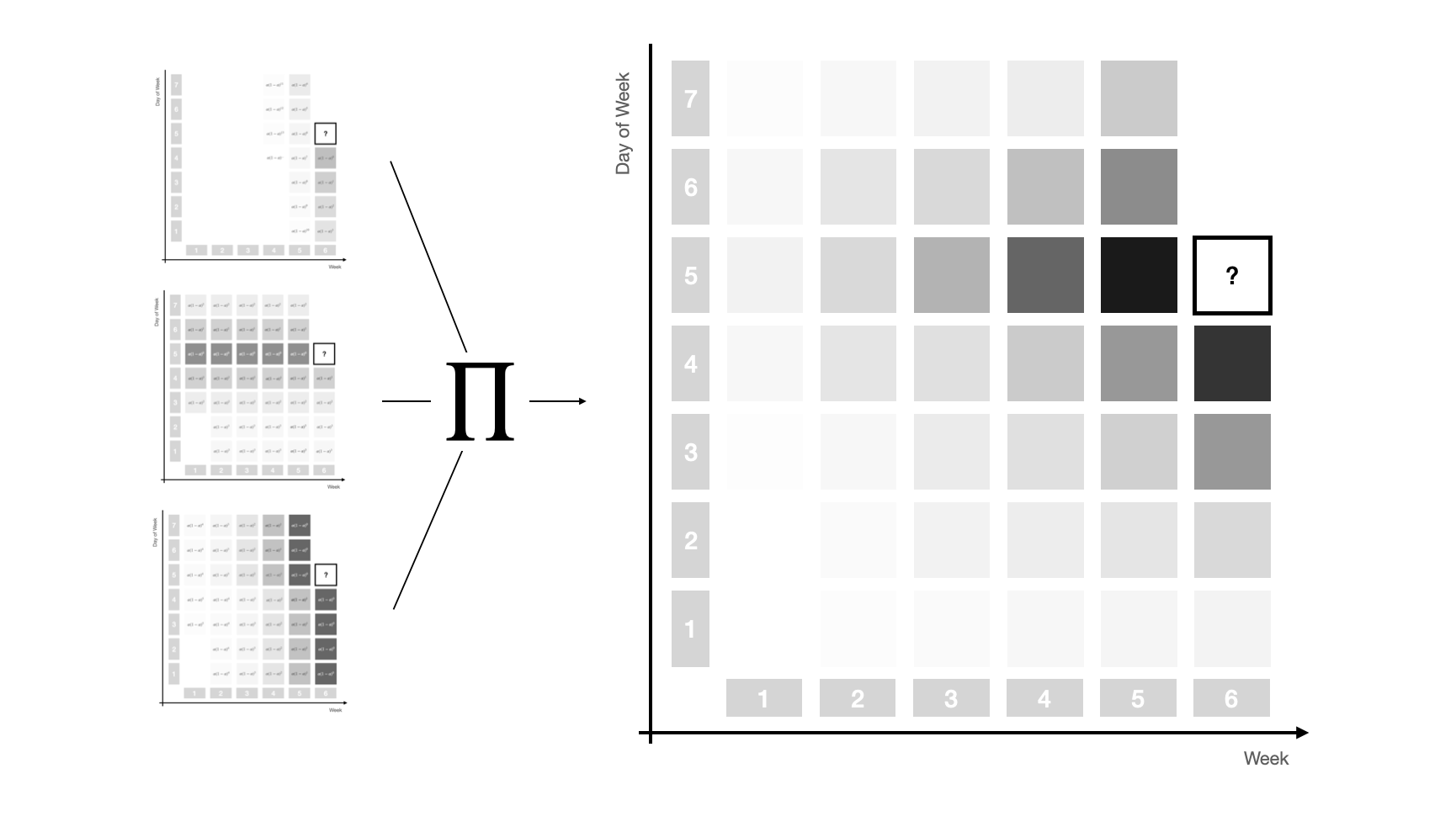
This three-dimensional exponential weighting structure captures the most important simple forecast methods as special cases. To make precise which set of parameters leads to which special case, let’s define a specific set of weights by the triplet \((\alpha, \alpha_{s}, \alpha_{sd})\).
Then, taking the average of weighted observations recovers
- the Naive method when all weight is assigned to the most recent observation \((1, 0, 0)\)
- the Mean method when equal weight is assigned to all observations \((0, 0, 0)\),
but due to the additional seasonal structures it now also recovers
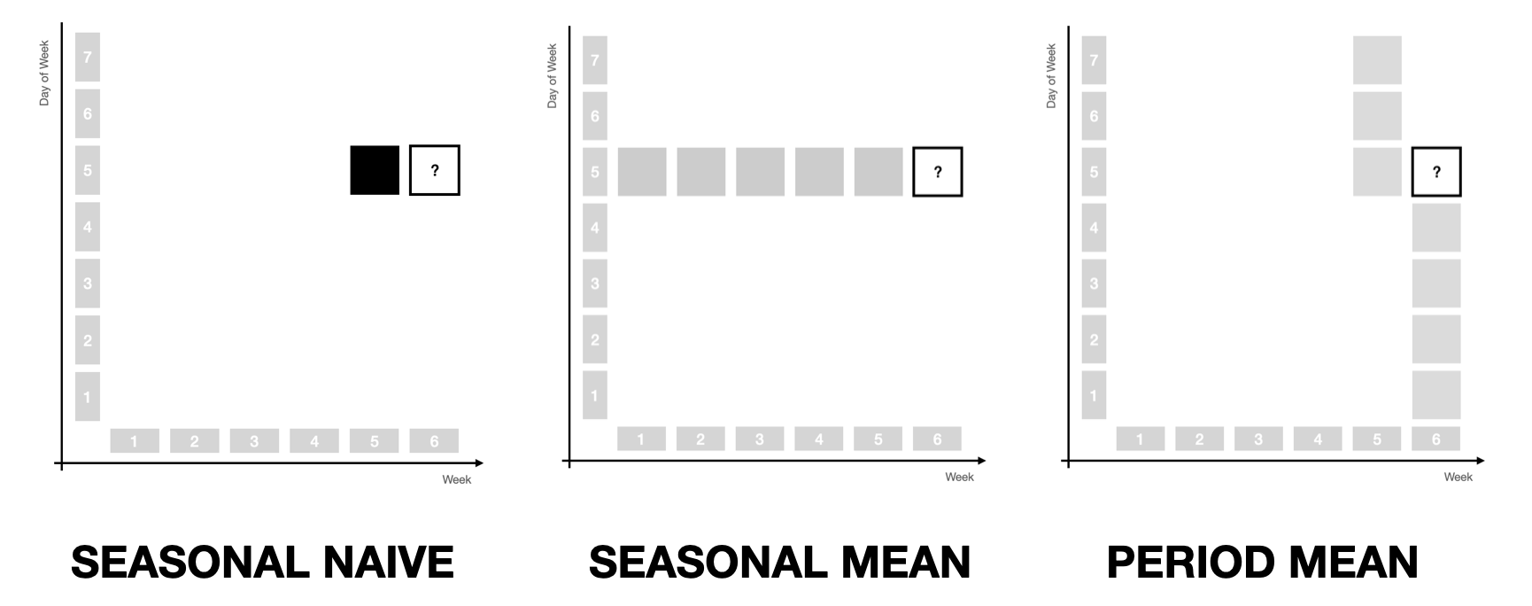
- the Seasonal Naive method when all weight is assigned to the observation a year ago \((0, 1, 1)\)
- the Seasonal Mean method when equal weight is assigned to only the same months in the past \((0, 1, 0)\)
- the Latest Period Mean method when equal weight is assigned to only observations from the twelve most recent months \((0, 0, 1)\).
The three latter cases are illustrated below.
Characteristics of the Model Family
What’s neat about this generalization of simple forecast methods is how the models built from the three parameter structure maintain the advantages of the simple methods that are found at the edges of the parameter space.
The reason for this is that we only apply weights to past observations in order to derive weighted average predictions.
For one, this implies that the models are robust in that they won’t predict outside the observed range of observations. In fact, you can think of them as regularized, stationary infinite-order AR models. While this is limiting when time series have sustained trends as their dominating signal, it also means that models won’t project a trend into the future by mistake. Depending on your data and the level of automation, this can be preferable.2
For another, any model in this family of models is perfectly interpretable. In fact, all you need to understand how a prediction is formed is to look at the weights allocated to past observations. It doesn’t get more interpretable than that. Even ETS models are hard to understand in comparison: Which observations made us predict that trend into the future again?
Finally, the three-dimensional exponential weights structure enables a range of possible adaptations.
For example, instead of creating probabilistic sample paths from a parametric distribution fitted to residuals (as is usual for the simple forecast methods mentioned before, as well as ARIMA and ETS, but also DeepAR in a sense), sample paths can also be drawn as a non-parametric bootstrap from the weighted observations, which can be helpful for intermittent and low-count data. This has been described in Gasthaus (2016) and Alexandrov et al. (2019) for the Non-Parametric Time Series Forecaster (NPTS) that is also available in AWS Forecast and GluonTS. In fact, the NPTS model can be described by the \((\alpha, 0, 0)\) and \((0, 1, \alpha)\) model specifications, depending on whether the non-seasonal or seasonal version is used.
Also, due to the parameter space’s simplicity, even brute force evaluation of parameter combinations is feasible to fit models. While a bit slower, it allows the use of any kind of loss function when fitting the model.
Implementation of the Model Family in threedx
Have a look at the threedx repository for an implementation and check out the corresponding website for more details and examples of how this model family based on weighting past observations can be used to forecast time series.
library(threedx)

y <- rpois(n = 55, lambda = pmax(0.1, 1 + 10 * sinpi(6:59 / 6)))

model <- threedx::learn_weights(
  y = y,
  period_length = 12L,
  alphas_grid = threedx::list_sampled_alphas(
    n_target = 1000L,
    include_edge_cases = TRUE
  ),
  loss_function = loss_mae
)

forecast <- predict(
  object = model,
  horizon = 12L,
  n_samples = 2500L,
  observation_driven = TRUE
)

autoplot(forecast)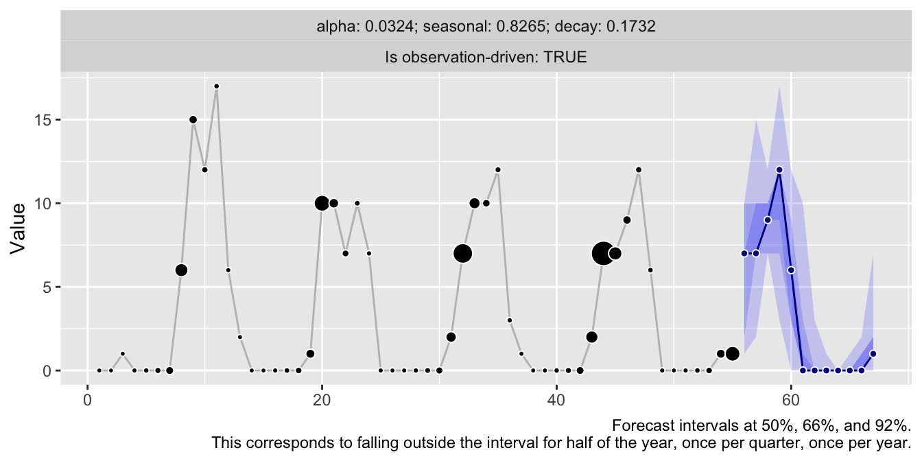
References
Alexander Alexandrov, Konstantinos Benidis, Michael Bohlke-Schneider, Valentin Flunkert, Jan Gasthaus, Tim Januschowski, Danielle C. Maddix, Syama Rangapuram, David Salinas, Jasper Schulz, Lorenzo Stella, Ali Caner Türkmen, Yuyang Wang (2019). GluonTS: Probabilistic Time Series Models in Python. https://arxiv.org/abs/1906.05264
Jan Gasthaus (2016). Non-parametric time series forecaster. Technical report, Amazon, 2016.
Rob J. Hyndman, Anne B. Koehler, Ralph D. Snyder, and Simone Grose (2002). A State Space Framework for Automatic Forecasting using Exponential Smoothing Methods. https://doi.org/10.1016/S0169-2070(01)00110-8
Vincent Warmerdam (2018). Winning with Simple, even Linear, Models. PyData London 2018. https://youtu.be/68ABAU_V8qI?feature=shared&t=286
P. R. Winters (1960). Forecasting Sales by Exponentially Weighted Moving Averages. https://doi.org/10.1287/mnsc.6.3.324
And, of course, subsequent standardization so they continue to sum to 1.↩︎
Additionally, there is always a possibility to project a bias in residuals created through a trend into the future when generating the forecast sample paths, as illustrated in this vignette.↩︎