Legible Forecasts, and Design for Contestability
Some models are inherently interpretable because one can read their decision boundary right off them. In fact, you could call them interpreted as there is nothing left for you to interpret: The entire model is written out for you to read.
For example, assume it’s July and we need to predict how many scoops of ice cream we’ll sell next month. The Seasonal Naive method tells us:
AS 12 MONTHS AGO IN August, PREDICT sales = 3021.Slightly more complicated but with rules that are fitted on past data, this is what a Rule List could look like:
     IF month IS June   THEN PREDICT sales = 5000,
ELSE IF month IS July   THEN PREDICT sales = 5900,
ELSE IF month IS August THEN PREDICT sales = 3050,
ELSE                         PREDICT sales = 1500.
The models are interpretable because their function \(f_{\theta}(x)\) is human-readable. The function is put into words, literally. This makes it possible to understand why a value is predicted, and it makes it possible to disagree with a prediction. A stakeholder could challenge it:
Yes, 3050 is a good estimate, but this August we run a discount code in our podcast advertisements for the first time ever, which is not taken into account by the model. Thus we should be prepared for increased sales of up to 4000 scoops of our delicious ice cream.
Users of interpretable methods can contest predictions because the models are legible. This is important, because methods that can be contested can also be trusted—basically every time you inspect the prediction and don’t find a reason to contest. I haven’t seen the terms “legible” and “contestability” mentioned a lot if at all in the usual machine learning literature around ethics, explainability, and trustworthiness. Instead a paper by Hirsch et al. on PubMed used them to describe a machine learning system built for mental health patients and practicioners. If you want others to trust and act on your model’s predictions, I think these are great characteristics to strive for.
Unfortunately, compared to the examples above, structural time series models aren’t legible. Or what do you call the following?
\[ y_{t} = \mu_t + \tau_t + \epsilon_t, \quad \epsilon_t \sim N(0, \sigma) \] \[ \mu_{t+1} = \mu_t + \delta_t + \eta_{\mu,t}, \quad \eta_{\mu,t} \sim N(0, \sigma_{\mu}) \] \[ \delta_{t+1} = D + \phi(\delta_t - D) + \eta_{\delta,t}, \quad \eta_{\delta,t} \sim N(0, \sigma_{\delta}) \] \[ \tau_{t+1} = - \sum_{s=1}^{S-1} \tau_t + \eta_{\tau, t}, \quad \eta_{\tau,t} \sim N(0, \sigma_{\tau}) \]
Sure, structural time series models are interpretable. That’s because they are made of a set of parameters where every parameter serves a predefined purpose. But it will take considerable effort and background knowledge to interpret not just individual parameters but all of them together to understand why the model predicts 3309 scoops of ice cream for August.
What though if we could write an interpreter for the coefficients? Not an explanation model that approximates the fitted model, but a function that puts the fitted parameters into words—again, the goal is legibility.
Let’s give it a shot.
Fit the Model
I will use the model described by the equations above for this. It’s implemented in the bsts package in R, and corresponds to the specification with semilocal linear trend and seasonal effects.

Photo of the bike counter installation at Straße des 17. Juni in Berlin. The counts of this station are available at: https://data.eco-counter.com/public2/?id=300019043.
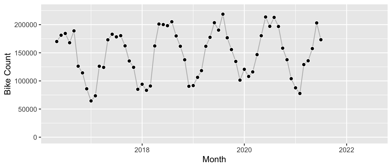
Let’s fit this model against monthly counts of bikes that passed the publicly available counter station at Maybachufer in Berlin; I aggregated the hourly data from the original dataset made available by the “Berlin Senatsverwaltung für Umwelt, Mobilität, Verbraucher- und Klimaschutz” on their website.1 It’s a smooth series of about five years history if we cut it off after June 2021 to keep a holdout year:
We construct the model by combining the semilocal linear trend with the monthly seasonality and fit it using the vector of the time series.
y <- df[df$date < as.Date("2021-08-01"), ]$n_bikes

state_spec <- bsts::AddSeasonal(
  state.specification = list(),
  y = y,
  nseasons = 12
)

state_spec <- bsts::AddSemilocalLinearTrend(
  state.specification = state_spec,
  y = y
)

bsts_fit <- bsts::bsts(
  formula = y,
  state.specification = state_spec,
  ping = 0,
  niter = 6000,
  seed = 7267
)
At this point we haven’t called predict() to produce a forecast. All we have are the fitted parameters of the model hidden in the bsts_fit object.2 Let’s plug them into our equation to print the model in the best form available out-of-the box:
\[ y_{t} = \mu_t + \tau_t + \epsilon_t, \quad \epsilon_t \sim N(0, 9290) \] \[ \mu_{t+1} = \mu_t + \delta_t + \eta_{\mu,t}, \quad \eta_{\mu,t} \sim N(0, 411) \] \[ \delta_{t+1} = -1.86 + -0.59 \cdot (\delta_t + 1.86) + \eta_{\delta,t}, \quad \eta_{\delta,t} \sim N(0, 8866) \] \[ \tau_{t+1} = \sum_{s=1}^{11} \tau_t + \eta_{\tau, t}, \quad \eta_{\tau,t} \sim N(0, 141) \] \[ \mu_T = 136570, \quad \delta_T = 3388 \] \[ \tau_T = 39881, \quad \sum_{s=1}^{11} \tau_{T-s+1} = 51118 \]
Well. I mean, one can interpret this. But would one show this as part of a user interface? Ask business stakeholders to make sense of it? Probably not. Can I type the values into a calculator and get the prediction for next month? Yes. Do I want to? No.
Make the Model Legible
Let’s try something different. In comparison to the numerical parameter values, a semantic representation should be much easier to parse. If there is one thing we can parse well, it’s text.3
The following function generates such legible representation of the fitted model, describes how the model puts the forecast together, and summarizes miscellaneous information such as comparison against benchmarks and detected anomalies.
Note that the paragraphs up to the horizontal divider below are automatically generated text returned by the function, based on the specifics of the model it received as input.
# devtools::install_github("timradtke/explainer")

explanation <- explainer::explain(
  object = bsts_fit,
  burn = 1000,
  seasonality = 12,
  start_period = 5
)
print(explanation)
The chosen model takes into account seasonality and allows for a long-run trend with short-term fluctuation around the trend.
The model explains most of the observed variation in the series at hand. This indicates that the series contains signals such as trend or seasonality, but it doesn’t guarantee that the model’s forecast projects them appropriately into the future.
Historically, the model has predicted the series at hand better than both the current year’s runrate, and the value from a year ago.
The current level of the series is lower than the average level observed in the history of the series, and lower than a year ago. The current level is neither clearly decreasing nor clearly increasing.
The model estimates a strong seasonal component in the series which will be projected into the future.
The model does not predict a clear upward or downward long-run trend.
The series’ seasonality is expected to push up next month’s observation, similar to a year ago.
Both observation noise and changes of the level of the series contribute to the forecast uncertainty. The level of the time series fluctuated historically both due to noise and due to changes in the trend.
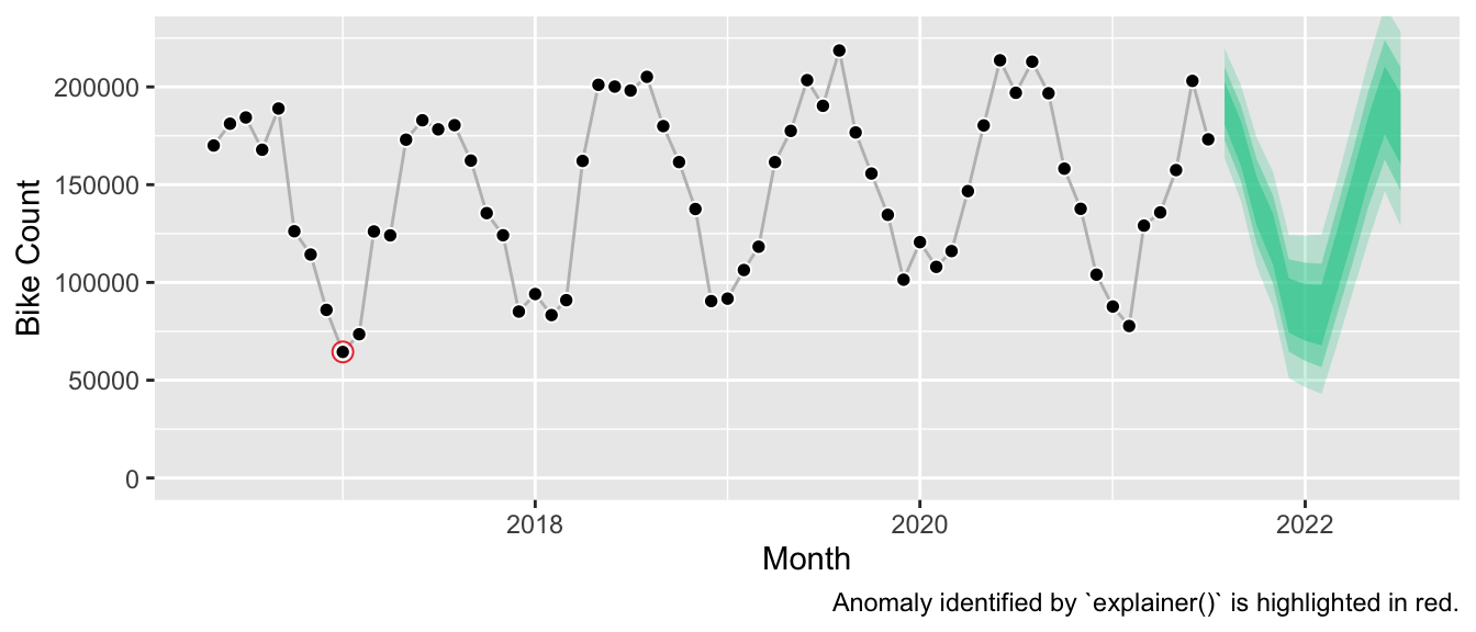
Over the course of the series, there has been a single anomaly 4.5 years ago.
This model representation isn’t as succinct as the set of equations. But you can read it from top to bottom. There’s no need to jump back and forth to grasp the size of the seasonal effect. It describes the characteristics of the fitted structural time series model without asking the reader to know what a structural time series model is. By doing so, it makes the model legible (literally), and contestable: For example, the model does not project a long-term trend (even though the model family allows for it). Given subject matter expertise, this could be challenged. Maybe 2020 and 2021 are unusual for some reason, and the upward behavior of the years prior will eventually continue.
What’s hidden in the function definition of explainer(), is that this interpretation relies on arbitrary thresholds. I purposely avoided printing any numbers to indicate the strength of model components. Consequently, it’s not left to the reader to determine whether the model shows a long term trend, whether the level is expected to increase, and which source of uncertainty is the strongest. It’s based on predefined cutoffs.
However, this allows us to play a bit with the information that is provided by the model object. Instead of purely interpreting the model parameters, one can expose how the model’s training (!) error compares to simple benchmarks like the seasonal naive method. If it compared unfavorably, this would presumably indicate that the model should not be relied upon. Similarly, the in-sample errors are used to identify potentially anomalous observations.4 Given the smooth bike counts, this isn’t as relevant here. But it could be valuable information to the user if a recent observation was unexpectedly large.
The Forecast
Finally, to complete the picture: The corresponding forecast looks as follows.
References
Tad Hirsch, Kritzia Merced, Shrikanth Narayanan, Zac E. Imel, David C. Atkins (2017). Designing Contestability: Interaction Design, Machine Learning, and Mental Health. DIS (Des Interact Syst Conf).
Fulton Wang, Cynthia Rudin (2015). Falling Rule Lists. Proceedings of the Eighteenth International Conference on Artificial Intelligence and Statistics.
Berlin Senatsverwaltung für Umwelt, Mobilität, Verbraucher- und Klimaschutz. Ergebnisse der automatischen Radzählstellen (Jahresdatei). 2021-12-31. Data licence Germany – attribution – version 2.0.
Their Excel file appears to be updated once a year which means the data for 2022 is not yet available. One can see the latest data on their interactive map.↩︎
As we used Bayesian inference, we don’t have a fitted parameter, but samples from parameters’ posterior distributions derived via MCMC. I will not mention it in the rest of the article and only show the posterior median.↩︎
Okay, after visual representations.↩︎
See also the documentation of
bsts::bsts.prediction.errrors().↩︎