Failure Modes of State Space Models

The Model

To keep it instructive and because the analysis extends to the other standard model families of Innovation State Space Models (as in forecast::ets(), for example) and Structural Time Series Models / Multiple Sources of Error State Space Models (as in bsts::bsts(), for example), let’s consider the univariate local level model.

Written as Structural Model, we have:

\[ y_t = l_{t-1} + \epsilon_t \]

\[ l_t = l_{t-1} + \eta_t \]

for the measurement and the transition equation, respectively, where

\[ \epsilon_t \sim N(0, \sigma_{\epsilon}) \]

\[ \eta_t \sim N(0, \sigma_{\eta}). \]

The equivalent model in Innovation State Space form can be written as:

\[ y_t = l_{t-1} + \epsilon_t \]

\[ l_t = l_{t-1} + \alpha \cdot \epsilon_t \]

where

\[ \epsilon_t \sim N(0, \sigma_{\epsilon}). \]

In the following we will focus on the Innovation State Space Model formulation as we use the forecast package to fit the model in our examples. However, the conclusions translate to the Structural Model as

\[ \alpha = - \frac{\sigma^2_{\eta}}{2\sigma^2_{\epsilon}} + \sqrt{(1 + \frac{\sigma^2_{\eta}}{2\sigma^2_{\epsilon}})^2-1} \]

for \(\alpha \in (0,1)\) as is the parameter space allowed by the forecast::ets() implementation. For details, see chapter 13.4 of Hyndman et al. (2008).

This local level model is equivalent to simple exponential smoothing. As such, it presents a trade-off between the two extremes of random walk and mean forecast models. The mean model implies a constant level that doesn’t change over time. The random walk model implies a level that adjusts fully to the most recent observation. The simple exponential smoothing forecast is a mix of the two: As \(\alpha\) tends towards 1, the resulting model adjusts more to the most recent observations, thus behaving similar to the random walk. Inversely, as \(\alpha\) tends to 0, the level is barely adjusted based on the most recent observations and equals instead the arithmetic mean of all observations.

Equivalently: If \(\sigma_{\epsilon}\) is larger then \(\sigma_{\eta}\), the model will dominantly be driven by the observation noise and tend to the global mean. But if \(\sigma_{\eta}\) is much larger than \(\sigma_{\epsilon}\), the model is driven by the innovation noise: The level adjusts a lot and dominates the observation noise, thus favoring a model more similar to a random walk.

These simple observations have strong implications as to how state space models behave in the presence of anomalies and structural breaks.

But let’s first look at an example series produced by this model.

#' Sample a Local-Level Time Series via Multiple Sources of Error
gen_ssm_series <- function(n, sigma_obs, sigma_level, l_0 = 0) {
  l_t <- rep(l_0, times = n + 1)
  y_t <- rep(NA, times = n + 1)
  
  for (i in 2:(n+1)) {
    l_t[i] <- l_t[i-1] + rnorm(n = 1, mean = 0, sd = sigma_level)
    y_t[i] <- l_t[i-1] + rnorm(n = 1, mean = 0, sd = sigma_obs)
  }
  
  return(y_t[-1])
}

We use \(\sigma_{\epsilon} = 1\) and \(\sigma_{\eta} = 1\) (equivalent to \(\alpha = 0.62\)) to generate a series based on equally strong measurement and transition noise.

library(ggplot2)
library(forecast)
set.seed(365)

df <- data.frame(
  index = 1:80,
  value = gen_ssm_series(n = 80, sigma_obs = 1, sigma_level = 1)
)

ggp_base <- ggplot(df, aes(x = index, y = value)) +
  geom_line(color = "grey") +
  geom_point(pch = 21, color = "white", fill = "black", cex = 2) +
  labs(x = "Index", y = "Value")
print(ggp_base)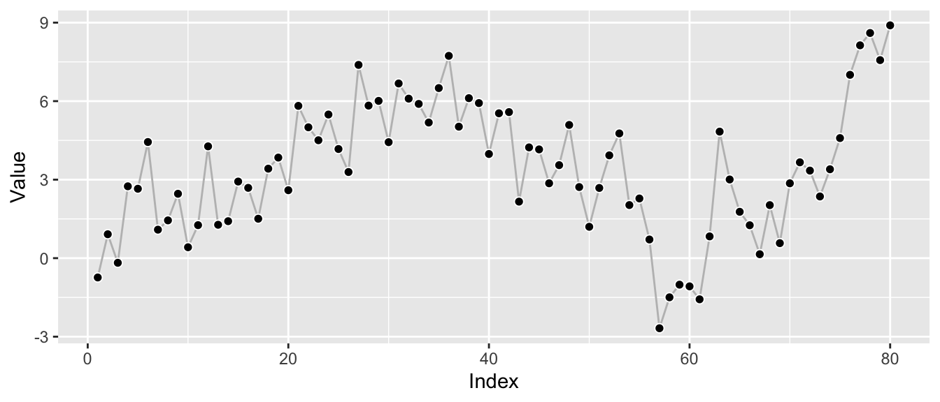

Knowing the true underlying model, we can fit a local-level model using the forecast package to try to recover the parameters.

ets_fit <- forecast::ets(y = df$value, model = "ANN")
print(ets_fit)

## ETS(A,N,N) 
## 
## Call:
##  forecast::ets(y = df$value, model = "ANN") 
## 
##   Smoothing parameters:
##     alpha = 0.618 
## 
##   Initial states:
##     l = -0.1009 
## 
##   sigma:  1.6243
## 
##      AIC     AICc      BIC 
## 432.1522 432.4680 439.2983

With alpha estimated as about the expected 0.62, the fitting procedure appears able to recover the underlying model well.¹ Let’s take a quick look at the corresponding forecast:

ggp_base + 
  autolayer(forecast::forecast(ets_fit, h = 12))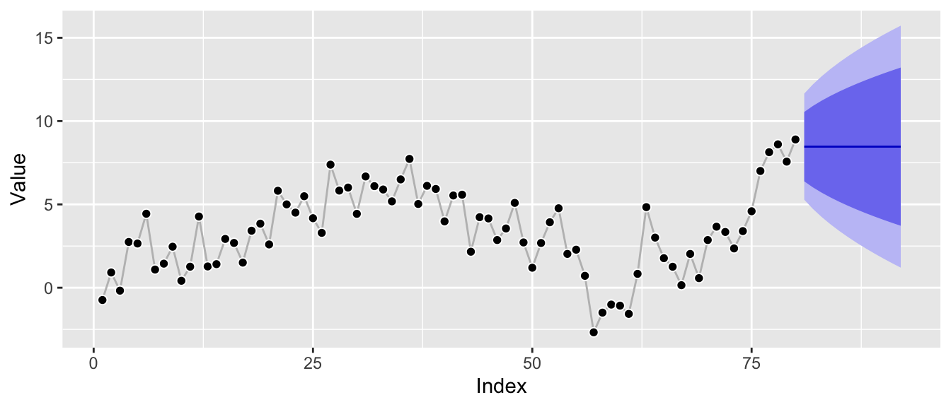

The model can be interpreted as interpolation between random walk and mean forecast, so it’s expected to be close to the recent level of the series. Additionally, the prediction intervals are increasing in width, but not as fast as those of a random walk model would, and clearly not constant as those of a mean forecast as the local level is expected to fluctuate in the future.

So far so good. Now how is this impacted by anomalies and structural breaks?

Cause for Trouble #1: Anomalies

Let’s consider an anomalous observation by adding it to the above series. To make the effect instructive, I won’t hold back—let’s make it really anomalous. This might look ridiculous, but believe me, this stuff exists.²

df_w_anomaly <- df
df_w_anomaly$value[55] <- df_w_anomaly$value[55] + 100

ggp_w_anomaly <- ggplot(df_w_anomaly, aes(x = index, y = value)) +
  geom_line(color = "grey") +
  geom_point(pch = 21, color = "white", fill = "black", cex = 2) +
  labs(x = "Index", y = "Value")
print(ggp_w_anomaly)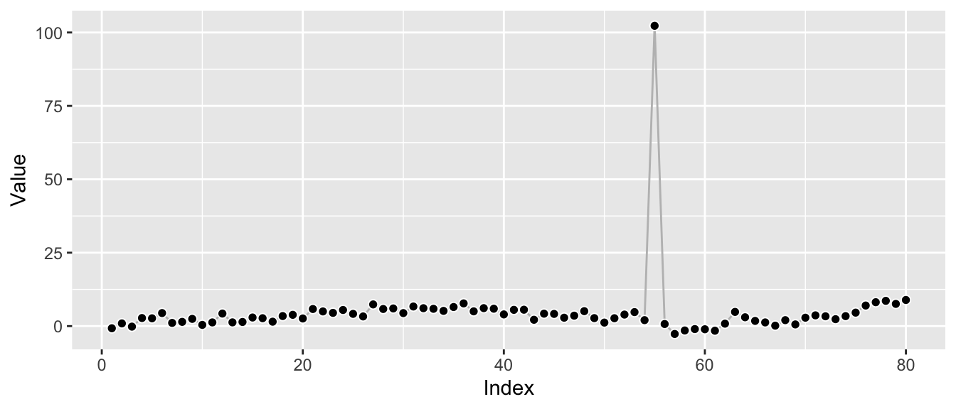

Let’s refit the model to consider the impact the anomaly has on the parameter estimates.

ets_fit_w_anomaly <- forecast::ets(y = df_w_anomaly$value, model = "ANN")
print(ets_fit_w_anomaly)

## ETS(A,N,N) 
## 
## Call:
##  forecast::ets(y = df_w_anomaly$value, model = "ANN") 
## 
##   Smoothing parameters:
##     alpha = 1e-04 
## 
##   Initial states:
##     l = 4.6512 
## 
##   sigma:  11.4091
## 
##      AIC     AICc      BIC 
## 744.0427 744.3584 751.1887

Remember that the original fit of the model above resulted in an alpha value of 0.62 which reflected the underlying local-level model. In contrast, the alpha value now dropped to 0: Instead of estimating a smooth interpolation of random walk and mean forecast, this alpha parameter corresponds to an essentially pure mean forecast.

This is immediately visible from the corresponding prediction intervals which are now constant:

ggp_w_anomaly + 
  autolayer(forecast::forecast(ets_fit_w_anomaly, h = 12))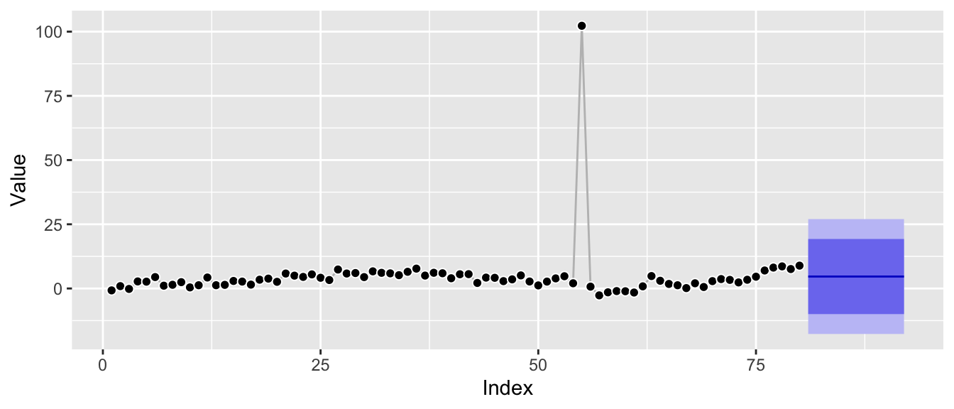

Zooming in to roughly the scale of the original plot it’s also clear that the underlying Gaussian distributional assumption translates the anomaly into much larger prediction intervals:

ggp_w_anomaly + 
  autolayer(forecast::forecast(ets_fit_w_anomaly, h = 12)) +
  coord_cartesian(ylim = c(-2.5, 15))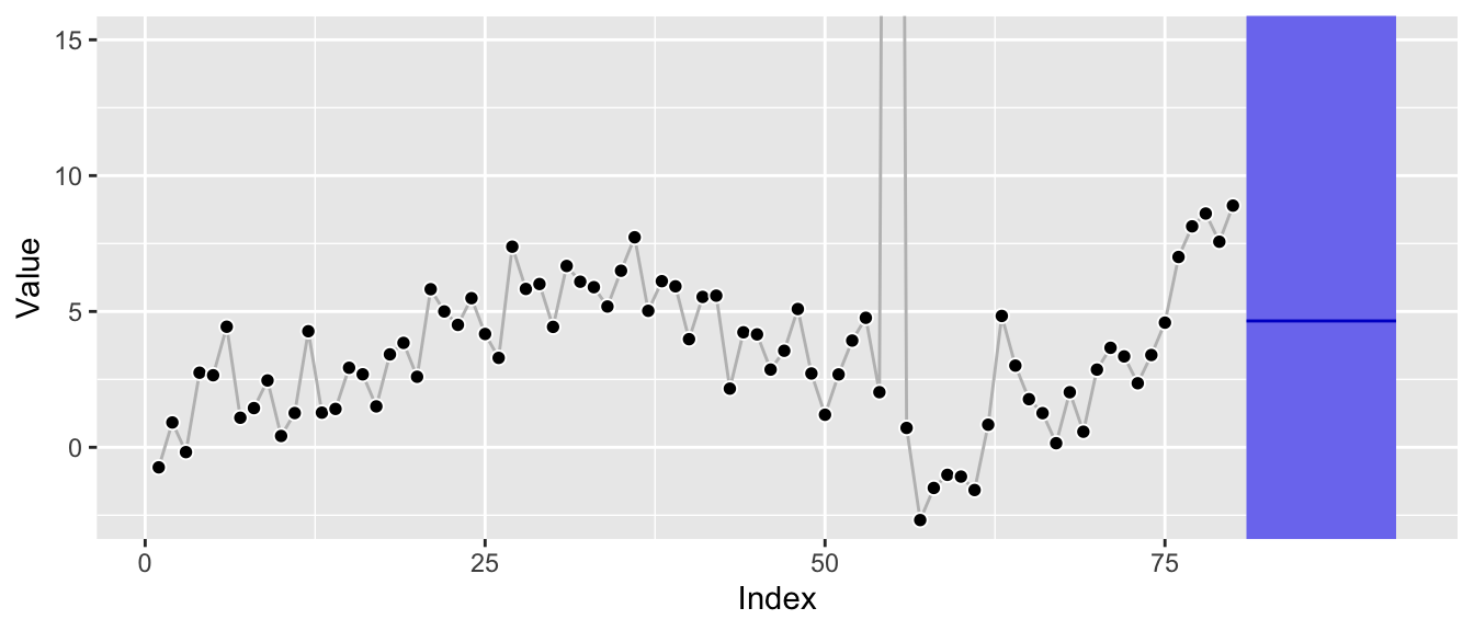

Additionally, the forecast is clearly biased away from the most recent level as the current level of the series is not equal to its global average.

Depending on the series itself and the size of the anomaly, a single anomaly leads the estimation procedure to choose an edge case of the structural time series parameter space, leading to poor forecasts.

The reason for this is simple: The mean forecast has the overall smallest (squared) errors once the anomaly is added. By choosing a mean forecast rather than something closer to a random walk, we only make the error introduced by the anomaly once, whereas a random walk would make it twice: Once for the anomaly itself, and then a second time right after the anomaly when jumping back to the actual level.

df_w_anomaly_residuals <- data.frame(
  index = rep(df_w_anomaly$index, times = 2),
  residuals = c(
    df_w_anomaly$value - mean(df_w_anomaly$value),
    df_w_anomaly$value - 
      c(NA, df_w_anomaly$value[-length(df_w_anomaly$index)])
  ),
  Model = rep(c("Mean", "Random Walk"), 
              each = length(df_w_anomaly$index))
)

ggplot(df_w_anomaly_residuals, aes(x = index, y = residuals)) +
  geom_line(color = "grey") +
  geom_point(pch = 21, color = "white", fill = "black", cex = 2) +
  labs(x = "Index", y = "Residual") +
  facet_wrap(~ Model)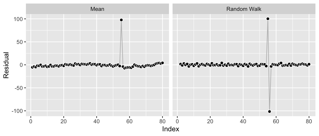

Let’s move on to the other cause for trouble: structural breaks.

Cause for Trouble #2: Structural Breaks

While there are many kinds of structural breaks, I’m concerned with level shifts here. This is a bit simplistic but instructive: Let’s shift the last 25 observations upward by a constant to introduce the shift for this example.

df_w_shift <- df
df_w_shift$value[55:80] <- df_w_shift$value[55:80] + 25

ggp_w_shift <- ggplot(df_w_shift, aes(x = index, y = value)) +
  geom_line(color = "grey") +
  geom_point(pch = 21, color = "white", fill = "black", cex = 2) +
  labs(x = "Index", y = "Value")
print(ggp_w_shift)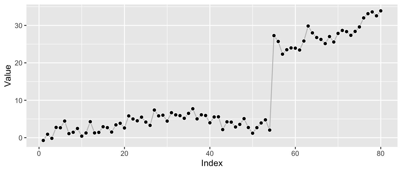

As before, let’s refit the model to consider the impact the level shift has on the parameter estimates.

ets_fit_w_shift <- forecast::ets(y = df_w_shift$value, model = "ANN")
print(ets_fit_w_shift)

## ETS(A,N,N) 
## 
## Call:
##  forecast::ets(y = df_w_shift$value, model = "ANN") 
## 
##   Smoothing parameters:
##     alpha = 0.7575 
## 
##   Initial states:
##     l = -0.3653 
## 
##   sigma:  3.2533
## 
##      AIC     AICc      BIC 
## 543.2815 543.5973 550.4275

The structural break leads to a new estimate of alpha at 0.76. Whereas the anomaly pushed the model towards a mean forecast, the level shift pushes it towards a random walk (though not all the way there) as that’s the model that adjusts quickest to the new level, thus avoiding the source of the single largest error in this data.

Again, this is visible from the residuals of the two edge cases:

df_w_shift_residuals <- data.frame(
  index = rep(df_w_shift$index, times = 2),
  residuals = c(
    df_w_shift$value - mean(df_w_shift$value),
    df_w_shift$value - 
      c(NA, df_w_shift$value[-length(df_w_shift$index)])
  ),
  Model = rep(c("Mean", "Random Walk"), 
              each = length(df_w_shift$index))
)

ggplot(df_w_shift_residuals, aes(x = index, y = residuals)) +
  geom_line(color = "grey") +
  geom_point(pch = 21, color = "white", fill = "black", cex = 2) +
  labs(x = "Index", y = "Residual") +
  facet_wrap(~ Model)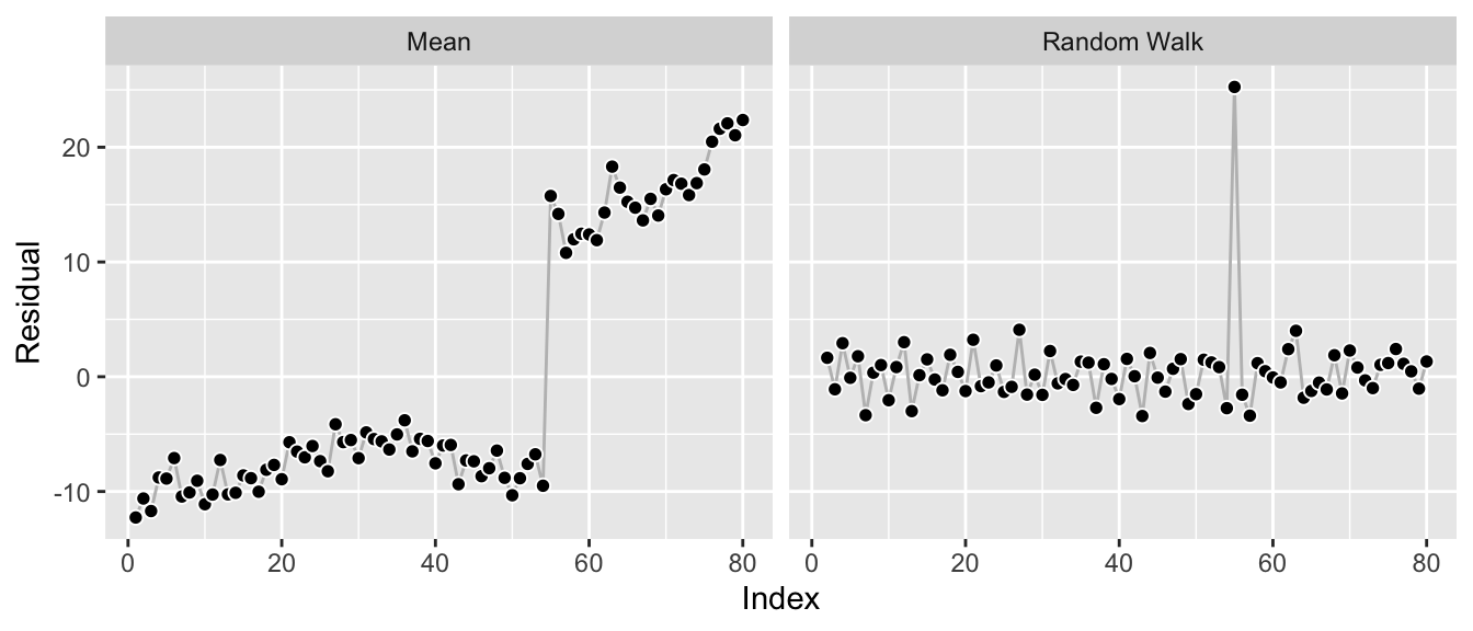

While the residuals look reasonable, a random walk forecast is not really ideal for the data. It’s good to model the shift, yes—but beyond that it leads to prediction intervals that are larger and growing faster than the period before the shift or the period after the shift would imply by themselves.

ggp_w_shift + 
  autolayer(forecast::forecast(ets_fit_w_shift, h = 12))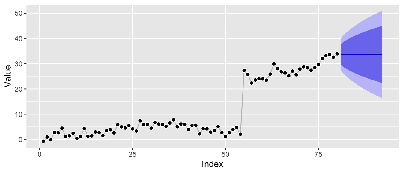

Everything Works as Intended

At this point, let me just reiterate that everything here works as intended.

Anomalies are just large observation noise so that’s what the model focuses on, resulting in a forecast dominated by observation noise—the mean forecast.

Level shifts are just large transition noise, so that’s what the model focuses on, resulting in a forecast dominated by transition noise—the random walk forecast.

If you use standard state space model implementations for your applications, you might as well write unit tests that check these behaviors and show them to your stakeholders. If your stakeholders’ time series show these patterns, then your models will adjust their forecasts accordingly.

Everything Works as Intended, and yet…

These fits frustrate me. The time series look good for the most part! But a single anomaly, a single level shift can mess the forecast up and make the forecast distribution useless.

With regard to anomalies, it would be nice to have model parameters that are robust against them but to reflect them properly in the uncertainty of the forecast. If we had fitted a model with alpha close to the original one but larger prediction intervals due to a larger sigma—that’s one thing. But the impact on the alpha and the corresponding bias of the forecast is not really acceptable. A low-hanging solution appears to be a different distributional assumption that replaces the Gaussian distribution as done in the models of the Orbit package. While this may fix the distorted sigma estimate, it won’t in general “fix” the smoothing parameters.

The level shift is also a bummer. Even forgetting the first half of the series and only using the observations after the shift would lead to a more appropriate model fit! But forgetting history is not something the state space models do: All observations are used to evaluate the likelihood, always.

Messy data needs messier models than the clean standard implementations with proven convergence behaviors.

References

Andrew C. Harvey (1990). Forecasting, Structural Time Series Models and the Kalman Filter. https://doi.org/10.1017/CBO9781107049994.

Rob Hyndman, Anne Koehler, Keith Ord, Ralph Snyder (2008). Forecasting with Exponential Smoothing: The State Space Approach. https://doi.org/10.1007/978-3-540-71918-2.

Edwin Ng, Zhishi Wang, Huigang Chen, Steve Yang, Slawek Smyl (2020). Orbit: Probabilistic Forecast with Exponential Smoothing. https://arxiv.org/abs/2004.08492.

Steven L. Scott (2017). Fitting Bayesian structural time series with the bsts R package. https://www.unofficialgoogledatascience.com/2017/07/fitting-bayesian-structural-time-series.html.