Pointwise Mutual Information for Instacart Product Recommendations
Using pointwise mutual information, we create highly efficient “customers who bought this item also bought” style product recommendations for more than 8000 Instacart products. The method can be implemented in a few lines of SQL yet produces high quality product suggestions. Check them out in this Shiny app.
Back in school, I was a big fan of the Detective Conan anime. For whatever reason, one of the episodes stuck with me. In that episode, the protagonists “pick up receipts in a convenience store to guess what the people are buying for dinner.” While this leads them inadvertently to a crime they need to solve, we will rather stick with the idea of finding out which products appear together in customers’ baskets.
Based on the Instacart Online Grocery Shopping dataset released a year ago, we analyze about 3 million orders of about 200,000 Instacart users. Similarly to how the detective boys used bought-together patterns to identify what customers were going to cook that evening, we’re going to find products that are bought together in order to create an effective, yet simple recommendation algorithm. So simple in fact, that the entire analysis could be productionized in plain SQL.
Instacart Data Set
From Wikipedia:
Instacart is an American company that operates as a same-day grocery delivery service. Customers select groceries through a web application from various retailers and delivered by a personal shopper.
The Instacart Online Grocery Shopping Dataset 2017 was made public by Instacart and can be downloaded here and offers a unique ability to try out recommendation algorithms on customer basket data. Then Instacart’s VP Data Science, Jeremy Kun introduced the data set in a Medium post. The dataset contains information on the products contained in about 3 million orders made by 200,000 Instacart customers. It thus lends itself as a testbed for machine learning methods that one would tend to apply at ecommerce companies–in particular those with a large variety of products, large basket sizes and returning customers.
Expected Result
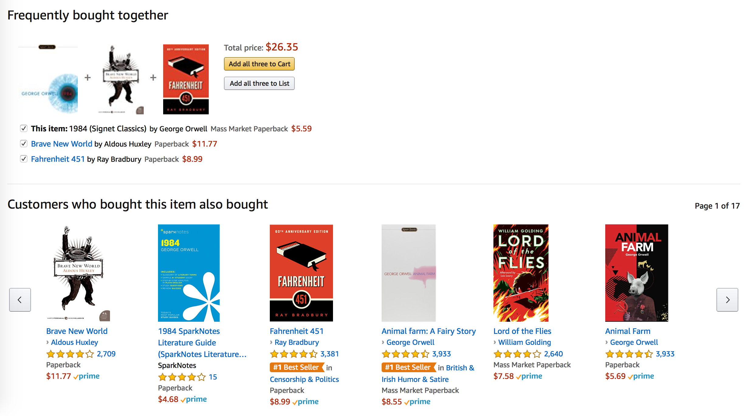
In his blog post, Jeremy Kun highlights how Instacart uses the data for example to sort their Buy It Again listings, or to model the Frequently Bought With recommendations. Here I will restrict myself to recommendations in the style of the latter. The results of the algorithm should be able to run under a “Frequently Bought Together” or “Customers Who Bought This Item Also Bought” headline. Much like Amazon’s famous recommendations, or the ones that Instacart employs itself.
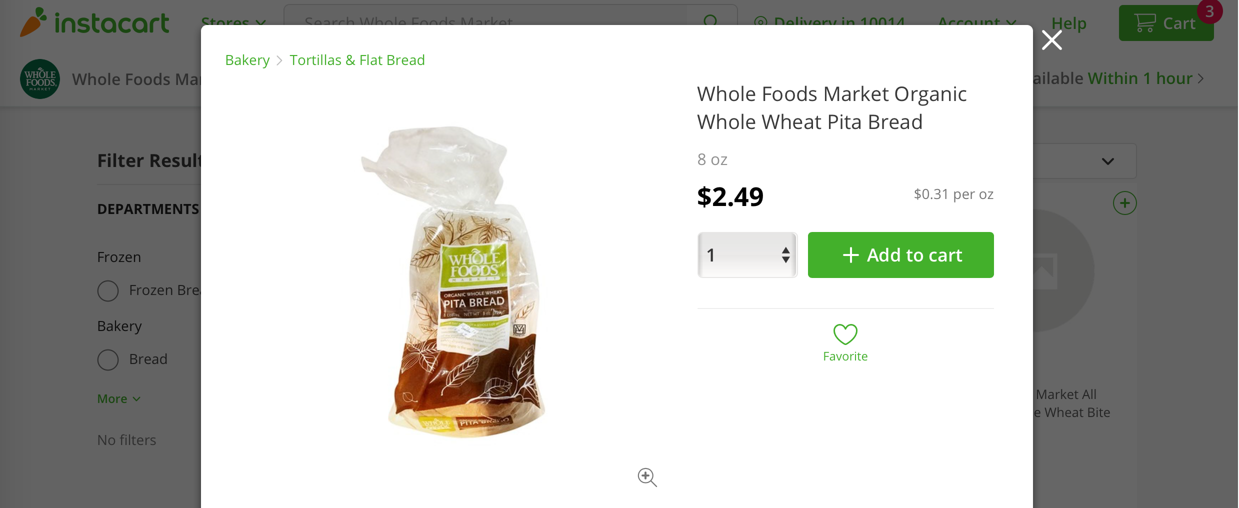
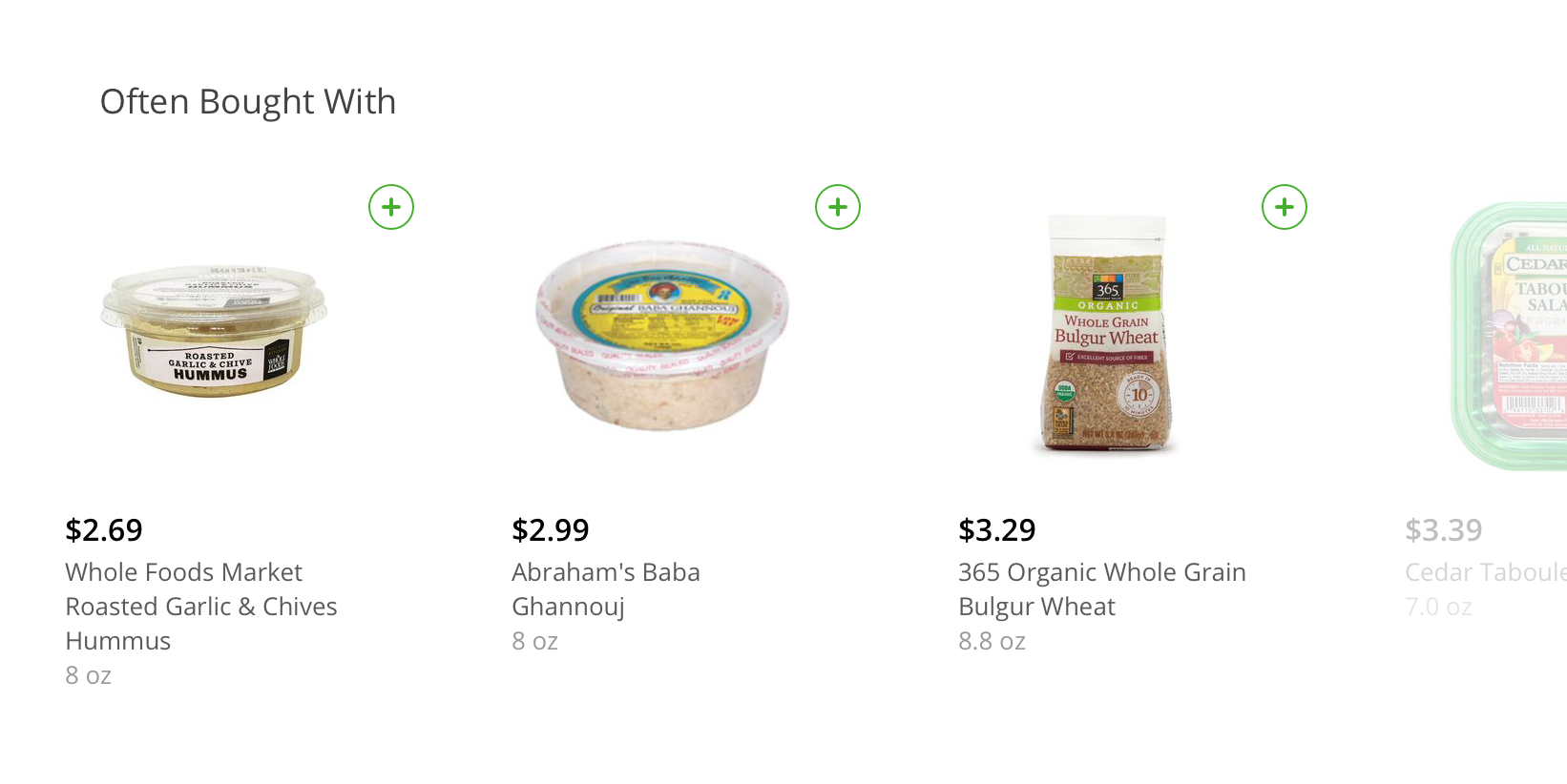
Take for example this Whole Foods pita bread offered on Instacart. Its page features recommendations for hummus and baba ghannouj under an “Often Bought With” headline, offering them as common complements. This style of recommendation is the goal, where we find items that go well together based on past purchases made by all customers. Those recommendations serve as a simple way for customers to fill their baskets with items that increase the value of the items they have already added to their baskets. It also ensures that customers don’t forget to buy items they really ought to buy.
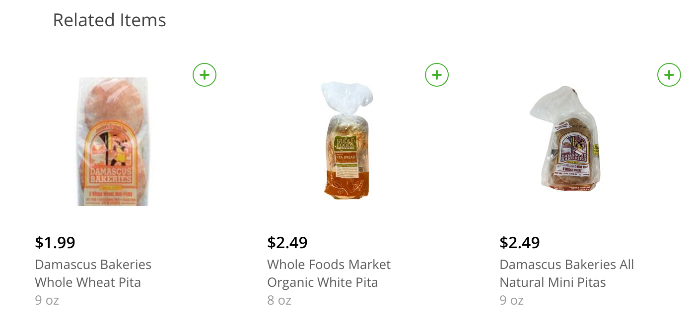
This stands in contrast to “Similar Items” or “Related Items” recommendations that are often found on the same product detail pages. These recommendations usually aim at direct substitutes to the product on the current detail page. On Instacart’s page for Whole Foods Market Organic Whole Wheat Pita Bread, I got served recommendations for a couple of other pita varieties, for example.
Methodology
So how exactly are we going to find the products that are often bought with pita bread? How do we know what customers who bought this item also bought?
The naive approach would be to count the pure item co-occurrence in orders: For every item, count how often it has been in an order with the pita bread, then recommend the item with the highest count. While this might surface a good recommendation from time to time, it will mostly surface bananas and toilet paper. Bananas and toilet paper are examples of a few very common items which appear in a large share of orders without being related to any product in particular. They would dominate any raw co-occurrence count just by their own purchase probability.
To account for this difficulty, we will make use of a simple trick from natural language processing: Pointwise Mutual Information.
Pointwise Mutual Information
Pointwise Mutual Information is a measure of association from information theory and has found a popular application in natural language processing. There, it measures the association between a word and the word’s context, e.g. close words in a sentence (bi-grams, n-grams, etc.). It does so by comparing how often the word and the context appear together against how often they would appear together were they independent events.
Following Wikipedia, we have for the outcomes \(x\) and \(c\) of two discrete random variables \(X\) and \(C\):
\[ pmi(x;c) = \log \frac{p(x,c)}{p(x)p(c)} \]
Here, the numerator describes the joint probability, while the denominator describes the joint probability under independence. Thus, were the two events independent, we would have \(pmi(x;c) = \log(1) = 0\). Consequently, positive PMI values imply positive association between the events (e.g., the word and its context, or between two products).
Similarly, negative PMI values should indicate negative relationships—but it’s generally not as easy to think in terms of words that do not appear together. While it’s easy to come up with co-occuring words (Google & Facebook, Scrum & Agile, Obama & Merkel), I failed to quickly come up with examples for the opposite. It’s not how we’re tuned to think. Also, the necessary corpus to correctly measure the PMI of words that do not appear together is very, very large—because they don’t appear together (see this book chapter by Daniel Jurafsky and James H. Martin).
Implementation
Data Preparation
We’ll now prepare the Instacart data and apply the PMI measure on the observed orders to find products that have been bought together.
To follow along, download the csv files from Instacart. First, we load some libraries and read the csv files. Note that these are the only packages we’ll need. This goes to show that we can do the same analysis in SQL, even though what follows is written in R.
library(dplyr)
library(readr)

# this is on order level
orders <- read_csv("orders.csv")
# this is on product level
products <- read_csv("products.csv")
# this is on order-product level
order_products <- read_csv("order_products__prior.csv")
Note that we only read one of the available order_products tables, since we will not perform an evaluation based on a test set. The orders table, however, contains information on more orders than those contained in order_products, so we slim it down:
# number of all orders
length(unique(orders$order_id))
## [1] 3421083# number of orders in our subset
length(unique(order_products$order_id))## [1] 3214874# we focus on the "prior" evaluation set for now
orders <- orders %>%
filter(eval_set == "prior") %>%
select(-eval_set)In the next few steps, we trim down the set of considered customers and products to only include those for which we have enough observations.
# first, get for every user his number of orders
users <- orders %>%
  group_by(user_id) %>%
  summarize(orders = n())
summary(users$orders)
## Min. 1st Qu. Median Mean 3rd Qu. Max.
## 3.00 5.00 9.00 15.59 19.00 99.00# drop all users who had a single order or a very large number of orders
# (customers who only made one order might have bought "trial baskets")
good_users <- users %>%
filter(orders <= 50, orders >= 1) %>%
pull(user_id)
# filter for the corresponding orders
good_orders <- orders %>%
filter(user_id %in% good_users)
# count for every user the number of different items he bought
product_by_customer_count <- order_products %>%
inner_join(select(good_orders, order_id, user_id)) %>%
distinct(user_id, product_id) %>%
count(product_id)
# A considered product should have been bought by
# at least 0.1% of the customers
product_threshold <- length(unique(good_orders$user_id)) * 0.001
good_products <- product_by_customer_count %>%
filter(n >= product_threshold) %>%
pull(product_id)
op <- order_products %>%
select(order_id, product_id) %>%
inner_join(select(good_orders, order_id, user_id)) %>%
filter(product_id %in% good_products)
# as last step, exclude all orders with a basket size of 1
op_size_one <- op %>%
group_by(order_id) %>%
summarize(basket_size = n()) %>%
ungroup %>%
filter(basket_size == 1) %>%
pull(order_id)
op <- op %>%
filter(!(order_id %in% op_size_one))After this initial data cleaning, let’s see how many orders, users, and products we are dealing here:
length(unique(op$order_id))## [1] 2315386length(unique(op$user_id))## [1] 194760length(unique(op$product_id))## [1] 8979So after dropping some customers and orders, we are left with about 200k users who bought about 9000 different products across 2.3 million orders. That should more than suffice to compute some PMI values.
Pointwise Mutual Information for Instacart Products
To compute the PMI value for every product, we first of all need to count how often products appear together. For the dataset at hand, the following expansion of the order_products table works fine (you should have quite some RAM though…); for every order, we join every product against every product in the order. This makes our table much longer, so depending on the average basket size and number of orders in another dataset, it might be a prohibitively expensive computation. We then immediately count how often products appear together:
op_pp <- inner_join(op, op,
                    by = c(order_id = "order_id")) %>%
count(product_id.x, product_id.y)dim(op_pp)## [1] 31708163 3Next, we need to count how often every product appears in orders, generally. This is used to compute the probabilities \(p(x)\) and \(p(c)\). We add these counts to the co-occurrence counts, and add the number of total orders in the total_n column. At this point we have all ingredients to compute the empirical probabilities and the PMIs.
product_count_train <- op %>%
  count(product_id)

pp_common_count <- op_pp %>%
  inner_join(product_count_train, by = c(product_id.x = "product_id")) %>%
  inner_join(product_count_train, by = c(product_id.y = "product_id")) %>%
  rename(common_n = n.x, x_n = n.y, y_n = n) %>%
  # total number of orders considered
  mutate(total_n = length(unique(op$order_id)))
Computing the PMI is now as simple as dividing columns and taking the logarithm. We add the corresponding product names to analyze the results afterwards.
pp_pmi <- pp_common_count %>%
  mutate(common_freq = log(common_n / total_n),
         x_freq = log(x_n / total_n),
         y_freq = log((y_n / total_n)),
         pmi = common_freq - x_freq - y_freq)

pp_rec <- pp_pmi %>%
  select(product_id.x, product_id.y, total_n, common_n, x_n, y_n, pmi) %>%
  left_join(select(products, product_id, product_name),
            by = c(product_id.x = "product_id")) %>%
  left_join(select(products, product_id, product_name),
            by = c(product_id.y = "product_id"))
Detailed Look at Recommendations
Given that we have not exactly fitted a model here, it’s not clear how to evaluate the results. We’re not explicitly optimizing for anything, so the following evaluation will be restricted to looking at some recommendations and judging whether the recommendations “make sense”.1
Given the large sortiment, I had to pick some products at random to evaluate the recommendations. Also, I had to pick products that I actually know–I’m not living in the U.S., so what is Glacier Freeze Frost?
For a start, let’s act as if we are about to add Spicy Avocado Hummus to the cart. What could I buy with hummus? Apparently a lot of other hummus, yogurt, as well as crackers or chips:
pp_rec %>%
  filter(product_id.x == 5973, product_id.x != product_id.y) %>%
  arrange(-pmi) %>%
  top_n(10, pmi) %>%
  select(product_name.x, product_name.y, pmi, common_n, x_n, y_n) %>%
knitr::kable(digits = 2)| product_name.x | product_name.y | pmi | common_n | x_n | y_n |
|---|---|---|---|---|---|
| Spicy Avocado Hummus | Organic Jalapeno Cilantro Hummus | 4.70 | 118 | 2541 | 982 |
| Spicy Avocado Hummus | Organic Kale Pesto Hummus | 4.47 | 97 | 2541 | 1015 |
| Spicy Avocado Hummus | Organic Thai Coconut Curry Hummus | 4.32 | 78 | 2541 | 945 |
| Spicy Avocado Hummus | Organic Sriracha Hummus | 4.31 | 144 | 2541 | 1762 |
| Spicy Avocado Hummus | Hummus, Hope, Original Recipe | 3.71 | 206 | 2541 | 4572 |
| Spicy Avocado Hummus | Total 2% Lowfat Greek Yogurt with Honey | 3.12 | 12 | 2541 | 481 |
| Spicy Avocado Hummus | Organic Jalapeno Crackers | 3.11 | 12 | 2541 | 489 |
| Spicy Avocado Hummus | Chomperz Original Crunchy Seaweed Chips | 3.09 | 17 | 2541 | 707 |
| Spicy Avocado Hummus | Teriyaki Turkey Jerky | 3.06 | 11 | 2541 | 472 |
| Spicy Avocado Hummus | Soft Toothbrush | 3.03 | 9 | 2541 | 397 |
Observe how we don’t have the Hummus, Hope, Original Recipe as the top recommended product even though the avocado hummus was bought most often with it. That is because the PMI takes into account how often the two products appear in orders independently. We see that the Hummus, Hope, Original Recipe is quite popular, which is why the 206 common orders are not as impactful as the 118 orders together with Organic Jalapeno Cilantro Hummus for the PMI. And so we want to rank the jalapeno hummus higher.
Notice also how some recommendations are based on just 9, 11, 12, or 17 common orders. If we think about how many customers we have, 12 orders can be noise. The toothbrush, for example, does not look like a good recommendation. We will address this with a smoothing method in a minute.
If we pick a different hummus, Garlic Hummus, we get very different results. There is no other hummus recommended, and instead the recommendations focus on pita bread. But notice again how the PMI favors products with a small number of common orders.
| product_name.x | product_name.y | pmi | common_n | x_n | y_n |
|---|---|---|---|---|---|
| Garlic Hummus | Whole Wheat Pita | 2.76 | 23 | 6893 | 489 |
| Garlic Hummus | White Pita | 2.75 | 71 | 6893 | 1518 |
| Garlic Hummus | Peanut Butter Dark Chocolate Fruit & Nut Protein Bars | 2.62 | 15 | 6893 | 368 |
| Garlic Hummus | Gluten Free Black Bean and Quinoa Burrito | 2.53 | 18 | 6893 | 480 |
| Garlic Hummus | Organic Spinach & Potatoes 2, 6 Months+ | 2.50 | 18 | 6893 | 495 |
| Garlic Hummus | Turkey Meatball Bites | 2.50 | 13 | 6893 | 358 |
| Garlic Hummus | 100% Whole Wheat Hot Dog Buns | 2.46 | 23 | 6893 | 659 |
| Garlic Hummus | Organic White Pita Bread | 2.42 | 37 | 6893 | 1102 |
| Garlic Hummus | Lotus Forbidden Rice Ramen | 2.38 | 10 | 6893 | 312 |
| Garlic Hummus | Gochujang Fermented Garlic Chile Paste | 2.20 | 7 | 6893 | 260 |
Similarly, here are recommendations for products that go well with Granny Smith Apples.
| product_name.x | product_name.y | pmi | common_n | x_n | y_n |
|---|---|---|---|---|---|
| Granny Smith Apples | Royal Gala Apples | 2.24 | 238 | 27712 | 2127 |
| Granny Smith Apples | Bag of Red Delicious Apples | 2.00 | 74 | 27712 | 835 |
| Granny Smith Apples | Seedless Grapes Green | 1.98 | 34 | 27712 | 392 |
| Granny Smith Apples | Dark Chocolate Chili Almond Nuts & Spices | 1.96 | 34 | 27712 | 399 |
| Granny Smith Apples | Outshine Lime Fruit Bars | 1.95 | 55 | 27712 | 651 |
| Granny Smith Apples | Golden Delicious Apple | 1.95 | 359 | 27712 | 4258 |
| Granny Smith Apples | Braeburn Apple | 1.93 | 126 | 27712 | 1523 |
| Granny Smith Apples | Garlic Parmesan Deli Style Pretzel Crisps | 1.91 | 49 | 27712 | 606 |
| Granny Smith Apples | Bag of Oranges | 1.89 | 131 | 27712 | 1657 |
| Granny Smith Apples | Whole Frozen Strawberries | 1.88 | 35 | 27712 | 445 |
When you work yourself through a couple of examples, it might stand out to you that the PMI tends to favor products with a small probability, that is, rare products tend to be recommended more. This is not necessarily desired, in particular not from the standpoint of a business.
Context Distribution Smoothing
As explained in Jurafsky and Martin (2017) citing Levy at al. (2015), a simple way to address this bias is context distribution smoothing, where the context probability is raised to the power of \(\alpha\), where \(\alpha \in (0,1)\). Since, for example, \(0.1^{0.75} \approx 0.1778\), doing so increases the probability of the context, and consequently decreases the PMI.
While there is also an impact on events with larger probability, the effect on events with small probability can be more extreme as for example here, leading to a larger absolute discount of their PMI values:
\[ \log(0.25) - \log(0.5) - \log(0.3) \approx 0.511 \] \[ \log(0.01) - \log(0.5) - \log(0.01) \approx 0.693 \] \[ \log(0.25) - \log(0.5) - \log(0.3^{0.75}) \approx 0.210 \] \[ \log(0.01) - \log(0.5) - \log(0.01^{0.75}) \approx -0.458 \]
It also implies that everything that would have been perfectly independent previously does now become negatively associated:
\[ \log(0.25) - \log(0.5) - \log(0.5) = 0 \] \[ \log(0.25) - \log(0.5) - \log(0.5^{0.75}) \approx -0.173 \]
Setting this aside, the context distribution smoothing can help in many cases to make the top ranks more sensible by returning more mainstream results. We can add the exponent (here 0.75) and compare the results:
context_exponent <- 0.75
pp_pmi_smooth <- pp_common_count %>%
  # smooth using the prior
  mutate(common_freq = log(common_n / total_n),
         x_freq = log(x_n / total_n),
         y_freq = log((y_n / total_n)^context_exponent),
         pmi = common_freq - x_freq - y_freq)

pp_rec_smooth <- pp_pmi_smooth %>%
  select(product_id.x, product_id.y, total_n, common_n, x_n, y_n, pmi) %>%
  left_join(select(products, product_id, product_name),
            by = c(product_id.x = "product_id")) %>%
  left_join(select(products, product_id, product_name),
            by = c(product_id.y = "product_id"))
For the apples we can observe that the seedless grapes, the Dark Chocolate Chili Almond Nuts & Spices, as well as Outshine Lime Fruit Bars have all been replaced by more apples, and the most frequently purchased item of them all: bananas.
pp_rec_smooth %>%
  filter(product_id.x == 9387, product_id.x != product_id.y) %>%
  arrange(-pmi) %>%
  select(product_name.x, product_name.y, pmi, common_n, x_n, y_n) %>%
  head(10) %>%
knitr::kable(digits = 2)| product_name.x | product_name.y | pmi | common_n | x_n | y_n |
|---|---|---|---|---|---|
| Granny Smith Apples | Royal Gala Apples | 0.49 | 238 | 27712 | 2127 |
| Granny Smith Apples | Golden Delicious Apple | 0.38 | 359 | 27712 | 4258 |
| Granny Smith Apples | Gala Apples | 0.37 | 1061 | 27712 | 18335 |
| Granny Smith Apples | Banana | 0.25 | 8919 | 27712 | 365728 |
| Granny Smith Apples | Red Delicious Apple | 0.21 | 236 | 27712 | 3062 |
| Granny Smith Apples | Mandarins Bag | 0.20 | 295 | 27712 | 4175 |
| Granny Smith Apples | Bosc Pear | 0.15 | 301 | 27712 | 4578 |
| Granny Smith Apples | Braeburn Apple | 0.10 | 126 | 27712 | 1523 |
| Granny Smith Apples | Bag of Oranges | 0.08 | 131 | 27712 | 1657 |
| Granny Smith Apples | Organic Fuji Apple | 0.08 | 2156 | 27712 | 69495 |
We see a similar effect for the garlic hummus. Compared to the previous recommendations, we also observe that more of the recommended items now have larger common_n values, i.e., by introducing the smoothing, we have implicitly ensured that the ranking relies more on common purchases.
| product_name.x | product_name.y | pmi | common_n | x_n | y_n |
|---|---|---|---|---|---|
| Garlic Hummus | White Pita | 0.92 | 71 | 6893 | 1518 |
| Garlic Hummus | Sea Salt Pita Chips | 0.90 | 351 | 6893 | 13135 |
| Garlic Hummus | Jalapeno Hummus | 0.65 | 157 | 6893 | 6310 |
| Garlic Hummus | Whole Wheat Pita | 0.64 | 23 | 6893 | 489 |
| Garlic Hummus | Lemon Hummus | 0.59 | 250 | 6893 | 12625 |
| Garlic Hummus | Organic White Pita Bread | 0.51 | 37 | 6893 | 1102 |
| Garlic Hummus | Pita Chips Simply Naked | 0.48 | 175 | 6893 | 9110 |
| Garlic Hummus | Organic Peeled Whole Baby Carrots | 0.44 | 532 | 6893 | 42519 |
| Garlic Hummus | Peanut Butter Dark Chocolate Fruit & Nut Protein Bars | 0.43 | 15 | 6893 | 368 |
| Garlic Hummus | 100% Whole Wheat Hot Dog Buns | 0.42 | 23 | 6893 | 659 |
Why PMI and not Common Order Count?
To quickly show the impact of using pointwise mutual information to rank the recommendations instead of the raw count of common orders, consider the following example. If we use the pointwise mutual information to get products that are bought together with Birthday Candles, we will get the following items as the top recommendations. The lighter is a natural complement, and everything else is to prepare the cake on which the candles are placed:
| product_name.x | product_name.y | pmi | common_n | x_n | y_n |
|---|---|---|---|---|---|
| Birthday Candles | Classic Lighters | 2.69 | 4 | 208 | 331 |
| Birthday Candles | Super Moist Chocolate Fudge Cake Mix | 2.63 | 4 | 208 | 360 |
| Birthday Candles | Creamy Classic Vanilla Frosting | 2.55 | 3 | 208 | 273 |
| Birthday Candles | Rich and Creamy Milk Chocolate Frosting | 2.51 | 3 | 208 | 285 |
| Birthday Candles | Funfetti Premium Cake Mix With Candy Bits | 2.48 | 5 | 208 | 587 |
If we instead rank by the absolute count of common purchases, the recommended products would be the generally frequently purchased bananas, strawberries, etc., just as I alluded to in the beginning. This just goes to show that the raw count is not an alternative to come up with product recommendations.
| product_name.x | product_name.y | pmi | common_n | x_n | y_n |
|---|---|---|---|---|---|
| Birthday Candles | Banana | -0.78 | 24 | 208 | 365728 |
| Birthday Candles | Organic Strawberries | -0.69 | 16 | 208 | 189410 |
| Birthday Candles | Large Lemon | -0.74 | 11 | 208 | 122928 |
| Birthday Candles | Bag of Organic Bananas | -1.66 | 8 | 208 | 274515 |
| Birthday Candles | Strawberries | -1.00 | 8 | 208 | 113606 |
Closing Thoughts
Recommendations based on pointwise mutual information alone are of course not perfect. It’s easy to find cases in which seemingly random products are recommended based on a few common orders. It’s difficult to filter these cases out by setting some threshold on the common orders; three common orders can produce good recommendations depending on the product (just consider the Birthday Candles example above).
More, since we’re not training a model and optimizing a metric, there is no scalable way of evaluating the result. Without picking a few example products and comparing recommendations, it’s difficult to, for example, pick the optimal smoothing exponent.
But the PMI ranking serves as excellent baseline solution. Given that only four columns have to be counted, the above recommendations can be written in a couple of lines of SQL. It doesn’t take more than a morning to go from no recommendations to a good solution. The PMI gives a lot of bang for the buck.
Not only that, but the PMI is also a natural starting point for word embedding models. As indicated in the references below, one could for example extend the ranking here to a full product-product PMI matrix. This high dimensional matrix could then be reduced into a lower dimensional embedding using something as simple as singular value decomposition (see Chris Moody’s “Stop Using word2vec” post on the Stitchfix blog). A word embedding makes it easy to train other models, as for example a clustering to find groups of related products.
In any case, take a look at the recommendations from the PMI ranking. I have published an interactive Shiny app which lets you select different products to simulate what could be presented on product display pages. The context smoothing parameter is adjustable as well. Try it out here. And next time your company needs product recommendations, try this as a cheap and good baseline.
References
The Instacart Online Grocery Shopping Dataset 2017. Accessed from https://www.instacart.com/datasets/grocery-shopping-2017 on May 2, 2018.
Daniel Jurafsky and James H. Martin. Vector Semantics. Book chapter in Speech and Language Processing. Draft of August 7, 2017.
Omer Levy and Yoav Goldberg. Neural Word Embedding as Implicit Matrix Factorization. In Advances in Neural Information Processing Systems 27 (NIPS 2014).
Omer Levy, Yoav Goldberg and Ido Dagan. Improving Distributional Similarity with Lessons Learned from Word Embeddings. Transactions of the Association for Computational Linguistics, vol. 3, pp. 211–225, 2015.
Chris Moody. Stop Using word2vec. Blog post in Stitchfix’ MultiThreaded blog.
Tomas Mikolov, Ilya Sutskever, Kai Chen, Greg Corrado and Jeffrey Dean. Distributed Representations of Words and Phrases and their Compositionality.
An first alternative would be to compare recommendations we derive from this “training” against the product combinations that appear in a test set.↩