Taxi Pulse of New York City
I don’t know about you, but I think taxi data is fascinating. There is a lot you can do with the data sets as they usually contain observations on geolocation as well as time stamps besides other information, which makes them unique. Geolocation and timestamps alone, as well as the large number of observations in cities like New York enable you to create stunning visualizations that aren’t possible with any other set of data.
For example, it is possible to visualize the streets of New York by simply plotting the locations at which taxis have picked up customers. You can find the version that I’ve created in R here, which is based on the ideas of two others who have written their visualizations in C and Python, respectively.
Earlier this year, there have been two competitions on Kaggle for which the organization of ECML/PKDD provided a data set on taxis in Porto, Portugal. For the first competition users were asked to predict the remaining travel time of a taxi after a customer had been picked up. The second competition challenged Kaggle users to build a predictive framework able to infer the final destination of taxi rides based on their partial trajectories.
The latest use case I’ve come across is a visual comparison of Uber usage in different cities created by Uber’s engineering team. You can find their graphics and the accompanying article on their blog. Each of their graphics shows the amount of Uber trips depending on weekday and hour. The number of trips is compared within weekdays with high levels of usage displayed in a bright blue color.
Of course, the data the engineering team used is private to Uber which restricts one from recreating the exact graphics. But since New York’s Taxi and Limousine Commission (TLC) has publicized their data on taxi usage, I’m able to create a corresponding graphic based on taxi cab usage.
To do so, I access the TLC’s data set through Google BigQuery. That way, I don’t have to work with .csv files that are several GB large. Instead, I can simply use a SQL query to extract the data in the format that I prefer. In this case, I’m especially interested in the timestamp describing the time at which the taxi rides occured. Since I only want to count each ride once, I don’t use both pickup and dropoff times but only pickup times. Furthermore, I would like to aggregate the rides on an hourly basis. Thus, I strip away the minutes and seconds from the timestamp using the HOUR() function in BigQuery. Seperately, I extract the date of the ride with DATE(). Using these two new columns, I can group the observations by date and hour in order to count the rides that occurred during an hour of a certain day. Additionally, I have restricted the observations I use on the area of New York City that I used for my previous graphics.
As last time, I don’t download the data directly through the BigQuery web interface but use the bigrquery package to access BigQuery through R instead. Proceeding this way, I can directly store the data in a data frame and continue to work with it.
library(bigrquery)
project <- "nyc-taxi-data-1048"
taxiTimes <- "SELECT DATE(pickup_datetime) AS pickupDay, HOUR(pickup_datetime) AS
              pickupHour, COUNT(*) AS num_pickups FROM [nyc-tlc:yellow.trips_2015]
              WHERE (pickup_latitude BETWEEN 40.61 AND 40.91)  AND
              (pickup_longitude BETWEEN -74.06 AND -73.77) GROUP BY pickupDay,
              pickupHour ORDER BY pickupDay, pickupHour;"

taxi_df <- query_exec(taxiTimes, project = project, max_pages = Inf)
dim(taxi_df)
# 4344 3
The resulting data frame has three variables and 4344 observations (one observation for every hour during the months from January to June of 2015).
A quick look into my calendar reveals that the first day of 2015 has been a Thursday. Therefore I can add the name of the days to the data frame with the following commands:
days_df <- data.frame(days = rep(rep(c("Thursday", "Friday", "Saturday",
                                       "Sunday", "Monday", "Tuesday",
                                       "Wednesday"),
                                     each = 24), length.out = 4344))
taxi_df <- cbind(taxi_df,days_df)
Now I have all information in the data frame that I would like to display in my graphic. The last thing to do before creating the actual visualization is to group the observations a second time, this time by weekday. While doing so, I take the mean of rides that have occured on a certain day during a certain hour. In the end, my data frame should therefore have 168 observations: 24 observations for each of the 7 days of the week.
library(plyr)

meanRidesDay <- function (taxidf) {
  mean(taxidf$num_pickups)
}
ridesPerWeekdayUTC <- ddply(taxi_df, .(dayUTC, hourUTC), meanRidesDay)

# > head(ridesPerWeekdayUTC, 3)
#    dayUTC hourUTC              V1
# 1    Friday              0 17396.423
# 2    Friday              1  11161.115
# 3    Friday              2   7313.385
So far, so good. The data frame is ready to be plotted. It contains three variables: The weekday, the hour, and the average number of rides that occured during the day and hour. It’s easy to now plot weekdays on the horizontal axis, hours on the vertical axis, and to use the average rides to create a density plot.
The ggplot2 package provides the function to do so: geom_tile(). Given a data frame containing a row for each combination of the discrete value ranges on both axes (here, a combination of every day with every hour), it creates a rectangle for every observation so that the plotting area is filled with tiles, one tile per observation. The color of the tiles is determined by the third variable; here, the average number of rides. The more rides there are, the brighter the color appears.
ridesPerWeekdayUTC$hourUTC <- as.factor(ridesPerWeekdayUTC$hourUTC)
taxi_plot <- ggplot(data = ridesPerWeekdayUTC, aes(x = dayUTC, y = hourUTC))
taxi_plot + geom_tile(aes(fill=V1)) +
  scale_x_discrete(limits=c("Monday", "Tuesday", "Wednesday", "Thursday",
                            "Friday", "Saturday", "Sunday")) +
  scale_y_discrete(limits = rev(levels(ridesPerWeekdayUTC$hourUTC))) +
  scale_fill_gradient(low="R #090A1C", high="#1FBAD6", guide=FALSE) +
  ggtitle("New York") +
  theme(axis.ticks = element_blank(),
        panel.background = element_rect(fill="#09091A", color="#09091A"),
        panel.grid.major = element_blank(),
        panel.grid.minor = element_blank(),
        axis.text.x = element_text(face="bold", size=12, color="#C0C0C8"),
        axis.text.y = element_text(face="bold", size=12, color="#C0C0C8"),
        plot.title = element_text(face="bold", size=40, color="#C0C0C8", vjust=1.1),
        axis.title.x = element_blank(),
        axis.title.y = element_blank(),
        legend.title=element_blank(),
        plot.background = element_rect(
          fill = "#09091A",
          colour = "#09091A"))
The remaining options I use in combination with ggplot() are simply needed to adjust the appearance of the plot to that of Uber’s template. Of course, I do not have Uber’s signature font. But there also isn’t an option in the ggplot2 package that allows me to move the x-axis labels to the top of the plot.
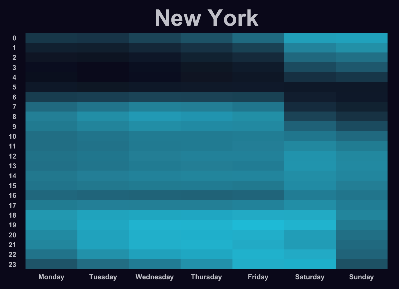
Looking at the result, the similiarity to Uber’s plot is obvious. Even though I use data on taxis for the first half of 2015, I am able to recreate the pattern that Uber has observed for New York with their 2014 data. Between 1am and 5am on Monday through Friday, the color is mostly black as even in New York most people are asleep. But there is a shift of this pattern on the weekend such that the number of taxis between 1am and 4am is noticeably higher. At the same time, people use the taxi regularly in the late evening except for on Sundays where they may prefer to stay at home. The same pattern is visible in Uber’s graphic for New York. Striking in my version might be the dark color for 4pm which is in contrast to 3pm and 5pm. This difference does not exist in Uber’s version.
Alas, I cannot create plots for different cities as Uber’s engineering team did. But I’m sure this hasn’t been the last time that I work with a taxi data set.