2026-11-07

Sample Path Evaluation

In my previous post, I attributed the lack of research into time series foundation models that forecast a joint distribution in part to the lack of benchmarks evaluating sample paths. You can’t claim state-of-the-art on forecast tasks that no one else evaluates themselves on. But claiming state-of-the-art matters. If GIFT-Eval, fev-bench, and TIME all evaluate quantiles of marginal distributions, then that’s what’s being built.

So be the change you want to see in the world. Build a sample path evaluation benchmark.

That’s what I did. Well, started. Prototyped. Considered: How could a benchmark for sample path evaluation look like?

I took the approach to sample path evaluation described in Bayesian Intermittent Demand Forecasting for Large Inventories (Seeger et al., 2016) and DeepAR: Probabilistic Forecasting with Autoregressive Recurrent Networks (Salinas et al., 2017) as a starting point. With the goal of using demand forecasts for inventory replenishment, the papers’ authors evaluate not (only) marginal forecasts but specific functionals of the joint forecast distribution relevant to their replenishment decisions. They evaluate, for example, the 90% quantile of the sum of daily forecasts of the twelve weeks following a lead time of three weeks (see Table 1 in Seeger et al.). This is the kind of aggregation I visualized previously:

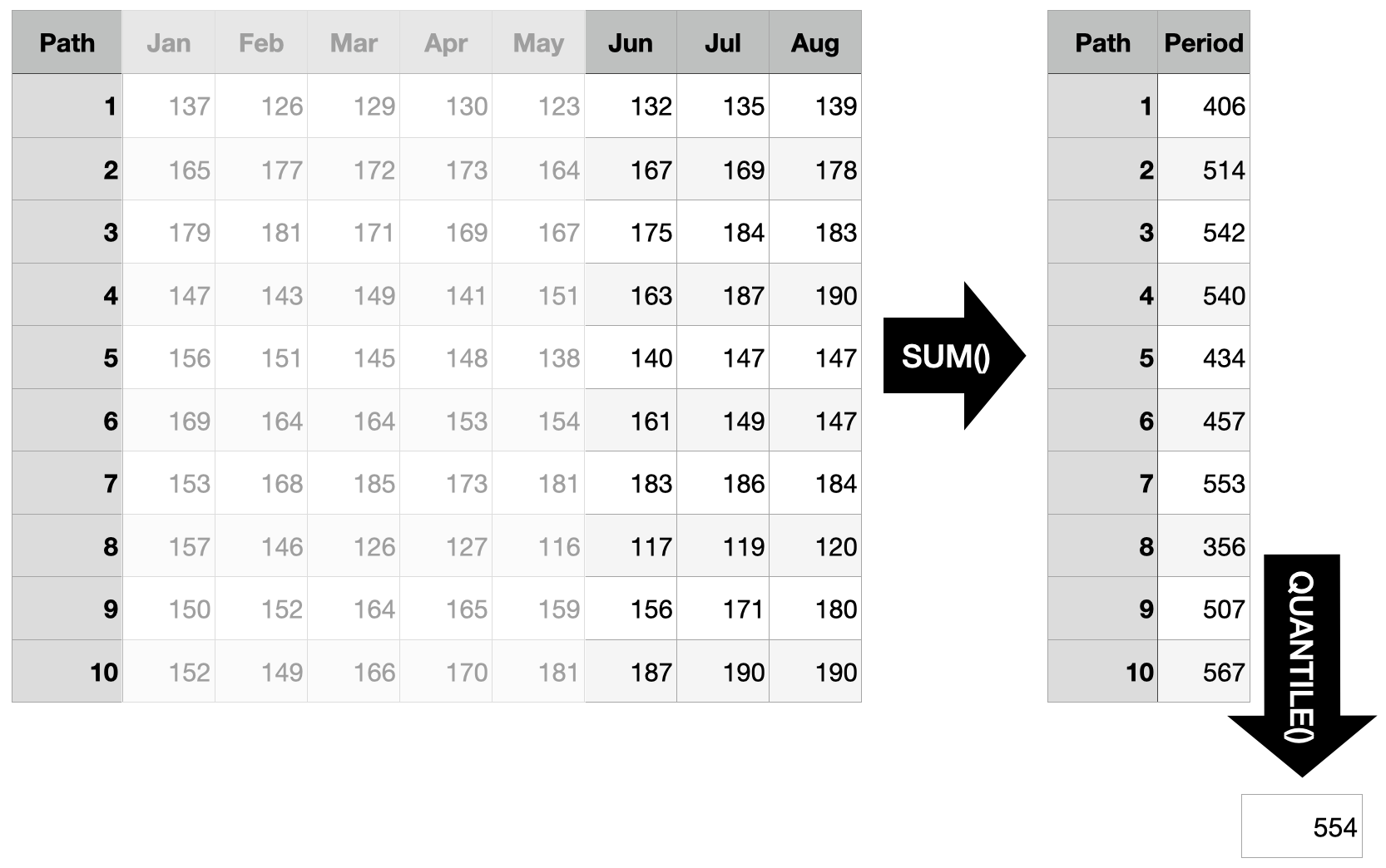
Aggregating forecasts of arbitrary points in time is crucial for replenishment decisions, and it requires forecasting the joint distribution over the forecast horizon. In lieu of closed form equations, sample paths make working with the joint distribution easy. To define these aggregates, the Seeger et al. and Salinas et al. parameterize them with a lead time and a span. Quoting Seeger et al. (2016):

Our metrics quantify the forecast accuracy of certain quantiles of predictive distributions. They are defined in terms of spans $[L,L+S)$ in the prediction range, where $L$ are lead times.

This approach to parameterizing aggregates of sample paths is what I used as one key ingredient to my proof of concept of an sample path evaluation benchmark. The other key ingredient was the fev package and its approach to defining forecast tasks and loading datasets for fev-bench.

Instead of rebuilding all that infrastructure, why not extend it. With spev (as in Sample Path EValuation), I extend a forecast task defined via fev by functionals of sample paths (such as the sum of a span following a lead time) and accompanying metrics. The metrics aren’t all that different from those already used by fev and other benchmarks. But I focus on quantile loss of individual quantile levels (such as the 90% quantile evaluated by Seeger et al.) and a CRPS calculated from samples instead of an approximation from quantiles.

Using spev then looks as follows. Import both fev and spev:

import numpy as np
from fev import Task
from spev import SamplePathTask

Then define a fev task that will serve as basis for the evaluation. Here, to both keep it simple and to reproduce the evaluation setup from Seeger et al. and Salinas et al., define the standard car parts task of forecasting the last eight months:

base_task = Task(
	dataset_path="autogluon/chronos_datasets",
	dataset_config="monash_car_parts",
	horizon=8,
	num_windows=1,
	seasonality=12,
	target="target",
)

Next, define a SamplePathTask by extending the Task. As described above, this implies defining aggregates and metrics. Here, I pick the ones from the papers:

task = SamplePathTask(
	base=base_task,
	aggregates=[
		{"name": "SUM", "lead_time": 0, "span": 1},
		{"name": "SUM", "lead_time": 2, "span": 1},
		{"name": "SUM", "lead_time": 0, "span": 8},
	],
	metrics=[
		# Mean Quantile Loss (Risk Score in the papers)
		{"name": "MQL", "quantile_level": 0.9},
		{"name": "MQL", "quantile_level": 0.5},
	]
)

With the task defined, draw some sample paths forecasts to evaluate.¹ The sample path forecasts need to be a list of one array per forecast window defined in the fev task (in this case, one window). Each array is four-dimensional: The first dimension is the number of time series, the second dimension is the number of samples, the third dimension is the length of the forecast horizon, and the fourth is the number of targets. In this case, the shape will be (2674, 2501, 8, 1).

rng = np.random.default_rng(seed=512)
sample_path_forecasts = [
	rng.poisson(
		lam=0.25,
		size=(
			2674, # Number of time series
			2501, # Number of sample paths
			8,    # Forecast horizon length
			1,    # Number of targets
		)
	)
]

Finally, pass the sample path forecasts to the spev task for evaluation. It returns a list of evaluated metrics, one for each combination of aggregates and metrics defined in the sample path task. Here, with 3 aggregates and 2 metrics, there are 6 evaluated metrics.

task.evaluation_summary(
	y_pred_per_window=sample_path_forecasts
)

[{'window': 0,
  'aggregate': 'Sum_[0,1]',
  'metric': '[email protected]',
  'value': array([1.40470307])},
 {'window': 0,
  'aggregate': 'Sum_[0,1]',
  'metric': '[email protected]',
  'value': array([0.47070546])},
 {'window': 0,
  'aggregate': 'Sum_[2,1]',
  'metric': '[email protected]',
  'value': array([1.44639299])},
 {'window': 0,
  'aggregate': 'Sum_[2,1]',
  'metric': '[email protected]',
  'value': array([0.47588681])},
 {'window': 0,
  'aggregate': 'Sum_[0,8]',
  'metric': '[email protected]',
  'value': array([4.12243922])},
 {'window': 0,
  'aggregate': 'Sum_[0,8]',
  'metric': '[email protected]',
  'value': array([2.79713033])}]

This result highlights an aspect that makes evaluating sample paths as part of a benchmark more uncomfortable than the evaluation of quantiles. Each aggregate multiplies the number of model comparisons.

But defining joint distribution forecast tasks is clearly possible. How fun would it be to have a benchmark of not only datasets from different domains, but also domain-specific aggregates and evaluation metrics. Use the SUM for inventory-related data, but the MAX for electricity load, or the ALL_GREATER_THAN for electricity prices.

Less one-size-fits-all, more sample paths.